The Description of Finite Sequential Processes

Kenneth E. Iverson
Harvard University, Massachusetts, U.S.A.^[a]
 

Introduction

The economical execution of fully-specified algorithms provided by the automatic computer has greatly increased the use of complex algorithms in information theory and other fields. This increased use has in turn generated a need for consistent and powerful programming languages for the description and analysis of complex algorithms. A programming language is commonly characterized as problem-oriented or machine-oriented, according as it is intended mainly for the description and analysis of algorithms or for their execution. The language outlined^[b] in the present paper was developed primarily for description and analysis, but also lends itself well to execution. The present emphasis is on description and analysis.

A programming language should (a) allow a clear and simple representation of the sequence in which steps of an algorithm are performed, (b) provide a concise and consistent notation for the operations occurring in a wide range of processes, (c) permit the description of a process to be independent of the choice of a particular representation for the data, (d) allow economy in operation symbols, and (e) provide convenient subordination of detail without loss of detail.

The sequence of execution of statements will be specified by their order of listing and by arrows connecting a statement to its successor. Branch points, at which alternative successors are chosen according to the outcome of a comparison between a pair of quantities, will be represented by a colon placed between the compared quantities, and by a label attached to each arrow showing the relation under which it is followed. Any well-defined relation may be employed, e.g. equality, inequality, or set membership. The conditions at each branch point must be exhaustive, and the listed successor is associated with all conditions not included in the labelled arrows.

Commonly occurring operations to be defined include the floor x (largest integer not exceeding x), the ceiling x, and the residue of x modulo m, to be denoted by |x, m|. The common logical operations and, or, and not will be denoted by ^, ∨, and ¯, and will be augmented by the relational statement (xR y) defined as follows. If x and y are any quantities and R is any binary relation defined upon them, then (xR y) is a logical variable whose value is 1 or 0 according as x does or does not stand in the relation R to y. For example, the absolute value of y may be defined as follows:

      |x| = x(1 - 2(x < 0))

To illustrate the use of the floor and ceiling operations, consider a rectangular array of dimension a × b whose cells listed in order by rows (0, 1, …, b – 1, b, b + 1, …, ab – 1) are denoted by x and in order by column are denoted by y. Then

      x = b × |y, a| + y ÷ a
and
      y = a × |x, b| + x ÷ b

These are the transformations used in determining accessibility in a serial-parallel memory of a bands with b slots per band. They may be derived from the identity

      y = a × y ÷ a + |y, a|
 

Ordered Sets

The description of a process can be made independent of its representation by defining certain fundamental operations upon finite ordered sets. The element of a finite simply ordered set B of dimension (number of elements) ν(B) can be indexed by the integers 1, 2, …, ν(B) such that B_i is the i-th element of the set. The k-th successor of an element x of B will then be denoted by x k and defined as the element B_j, where j ≡ (i + k) (mod ν(B)), and B_i = x. The k-th predecessor is defined analogously and denoted by x k. If B is the set of integers, the symbol B may be elided, and if k = 1 it may be elided; hence i↑k denotes the k-th successor of the integer i, and i ↑ denotes the integer i + 1.

The successor operation defined upon an element of B can be extended to any subset C of B as follows: C k denotes the set D such that D_i = C_i k. If C and B are identical, the operation is called left rotation and is denoted by C ↑ k. Rotation is extended analogously to vectors.

Two sets A and B are equal (A = B) if they contain the same elements, but are identical (A ≡ B) only if they also have the same order. Simple modifications in the standard definitions of intersection and union provide a closed system for ordered sets. To achieve economy of operation symbols, intersection and union are denoted by ^ and ∨, already used for the analogous logical operations and, and or. Potential ambiguity is avoided by using distinctive symbols for each class of operand; italics for single variables, lower case boldface italics for vectors, upper case boldface italics for matrices, and ordinary Roman characters for literals, i.e. for characters such as the numerals and the letters of the alphabet which have fixed accepted meanings.

A second set of indices, called contracurrent indices will be assigned to the elements of any set A. These indices run from –ν(A) to –1. The k-th element may therefore be denoted alternatively by A _k or A_–j, where j + k = ν(A) + 1. In particular, the terminal elements may be denoted by A₁ and A_–1. Contracurrent indices will also be employed for vectors and matrices.^[c]

A set obtained from a set B by deleting the first i and the last j elements is called a solid subset or an infix of B. An infix C of B is also called a prefix of B if C₁ = B₁, or a suffix if C_–1 = B_–1. The statement

      C {(x, y)}

specifies C as the infix of B having terminal elements x and y. The symbol B may be elided if B is the set of integers.

Program 1 illustrates the conventions introduced so far. If H _j¹ is the suit and H _j² the denomination of the j-th card in a hand of thirteen playing cards, and if

      D ≡ {deuce, trey, …, king, ace}

is the set of denominations, then the quantity q determined by the program is the length of the longest run in any one suit.

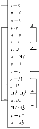Program 1. Program to determine the length of the longest run in the card hand H

A left-pointing arrow associates the specifying quantity on the right of each statement with the specified quantity on the left. The arrow is used instead of the sign of equality because it eliminates ambiguity and reserves the sign of equality as a relation to be used in relational statements only.
 

Structured Operands

Significant subordination of detail can be achieved by generalizing each operation defined upon simple variables to structured arrays such as vectors and matrices. For example, if p and q are logical vectors (i.e. each component is a logical variable), then

	r ←	↔	r i =  i		i ε {(1, ν(p))}
	r ← p ^ q	↔	r i = p i ^ q i
	r ← p ∨ q	↔	r i = p i ∨ q i

Moreover, if x and y are numerical vectors, then

Operations such as floor, ceiling, and residue are extended analogously.

The application of any associative binary operation to all components of a vector x is denoted by /x. Thus ×/x is the product and +/x is the sum of all components of x. The latter will also be denoted by σ(x) and be called the weight of x. The usual notations for matrix algebra are retained, i.e. xy for a scalar product, and XY for a product of matrices. It is clear that xy = σ(x × y) and that σ(x ↑ k) = σ(x) for all k.

Greek symbols (in the appropriate type face) will be used for specially defined quantities. Thus, the unit vectors ∊ⁱ are logical vectors such that (∊ⁱ) _j = 1 if and only if j = i. The full vector ∊ is the negation of the zero vector. The prefix vector ⍺ⁱ is a logical vector of weight j whose first j components are unity. The suffix vector ⍵ⁱ is defined analogously. The identity permutation vector ⍳ is defined by the relation ⍳ _j = j. The dimension of a unit, suffix, prefix, or identity permutation vector is normally defined implicitly by the compatibility requirements of associated operators and operands. The scalar zero, vector zero, and matrix zero will all be denoted by 0.

The conventional vector product of two space vectors (to be denoted by x y) will illustrate the use of the foregoing notation. It can be defined as

      x y = x ↑ × y ↓ – x ↓ × y ↑

A trivial formal manipulation shows that y x = –(x y). The orthogonality theorem x(x y) = 0 can be established as follows:

	x(x y)	=	x(x ↑ × y ↓ – x ↓ × y ↑)
		=	σ(x × x ↑ × y ↓ – x × x ↓ × y ↑)
		=	σ((x × x ↑ × y ↓) ↓ – x × x ↓ × y ↑)
		=	σ(x ↓ × x × y ↓ 2 – x × x ↓ × y ↑)

Since the × operator is commutative, and since y ↓ 2 = y ↑ for a vector of dimension three, the final expression is equal to zero and the theorem is established. Further theorems concerning the magnitude of x y, the four-vector product, and the box product follow by similarly simple formal manipulation.

Individual components of structured operands can be selected by subscripts and superscripts: x _i for the i-th component of the vector x, Aⁱ for the i-th row vector of a matrix A, A _j for the j-th column vector, and A _j ⁱ for the ij-th element. More generally, it is necessary to specify selected subsets of the components. Since the selection is, for each component, a binary operation, it can be specified by an associated logical vector of the same dimension. Thus for an arbitrary vector x and compatible logical vector u (that is, ν(u) = ν(x)), the statement

      z ← u/x

implies that the z is obtained by suppressing from x those components x _i for which u _i = 0. The operation u/x is called compression of x by u. For example, if u = (1, 0, 0,0, 1, 1), and x = (m, o, n, d, a, y), then u/x = (m, a, y). Clearly, ν(u/x) = σ(u). Set compression is defined analogously.

Two types of compression must be defined for matrices; row compression, defined by

For example, if the matrix M represents a ledger of μ(M) bank accounts, with the column vectors M₁, M₂, M₃, and M₄ denoting name, account number, address, and balance, respectively, then the operation of preparing a list P of the name, account number and balance, for all accounts whose balance exceeds 1,000 can be completely prescribed as follows.

      P ← (M₄ > 1000∊)//(³/M)

The expansion of a vector x by a logical vector u is denoted by u\x and is defined as follows.

      z ← u\x   ↔   u/z = x and /x = 0

It is necessary that σ(u) = ν(x). Clearly ν(z) = ν(u). Row expansion (denoted by u\X) and column expansion (u\\X) are defined analogously.

The compress and expand operations provide a powerful extension of ordinary matrix algebra. For example, any numerical vector can be decomposed according to the identity

      x = \/x + u\u/x

Matrices can be decomposed similarly. Moreover, the conventional operations on partitioned matrices can be generalized in a systematic manner. A few of the more important identities are, for example:

	(u/X)Y	=	X(u\\Y)
	(u\X)Y	=	X(u//Y)
	XY	=	(u/X)(u//Y) + (/X)(//Y)
	u/(XY)	=	X(u/Y)
	u//(XY)	=	(u//X)Y
	(u/v)/(u/X)	=	(u ^ v)/X

Maximization over those components of x for which u _j = 1 will be denoted by u⌈x. More precisely,

      v ← u⌈x

specifies a logical vector v such that v/x = m∊ and that

      (((v ^ u)/x) < m∊) = ∊

Graphically, v is obtained by lowering a horizontal line over a plot of x until it touches the largest component of u/x, and then marking with a 1 all components of u/x touched by the line. Thus if x = (6, 3, –8, 6, 6), then v = ∊⌈x = (1,0, 0, 1, 1), v/x = (6, 6, 6), and (v/x)₁ = 6. Minimization is denoted analogously by u⌊x. The minimum over all positive values of x may be denoted, for example, by (x > 0)⌊x, and for the present example (x > 0)⌊x = (0, 1, 0, 0, 0).

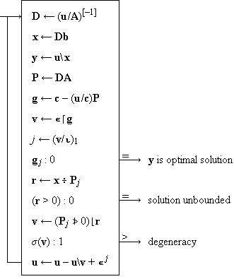Program 2. Complete program for the simplex algorithm of linear programming

The vector y determined is the optimal solution of the following system: maximize cy subject to the constraints (Ay ≤ b) = ∊, and (y ≥ 0) = ∊. The logical vector u is assumed to be given initially and specifies the current feasible basis; x is the corresponding vector of non-zero variables. A power of a matrix is denoted by a superscript enclosed in square brackets.

The operations occurring in Program 2 can be used in a formal analysis of its behaviour, For example,

      u/P = u/((u/A)^[–1] A) = (u/A)^[–1] (u/A) = I

and P therefore contains an identity matrix I in the columns corresponding to the feasible basis u. Moreover, since

      g = c – (u/c)P

      u/g = u/c – u/(u/c)P = u/c – (u/c)(u/P) = u/c – (u/c)I = 0

Hence the components of the modified cost function g are zero for all included variables, as desired.

The base b value of the vector x is denoted by b ⊥ x and defined as the value of x in the mixed base number system defined by the radices b₁, b₂, … b_–1. More precisely, b ⊥ x = xz, where z _–1 = 1 and z _–i = ×/(⍵ ^i–1/b), for i ε {(2, ν(b))}. If, for example, b = (7, 24, 60, 60), and x denotes elapsed time in days, hours, minutes and seconds, then b ⊥ x denotes the elapsed time in seconds. In particular, 10∊ ⊥ x denotes the value of x in the decimal system, and y∊ ⊥ x denotes the polynomial in y whose coefficients are the components of x.

For example, the standard single-error-correcting Hamming code for n binary digits can be described by a logical matrix U such that ν(U) = n, μ(U) = log₂(n + 1), and 2∊ ⊥ U _j = j. The i-th parity check group then includes the components of the vector U ⁱ/x and Program 3 describes the determination of the corrected value y of the code x. An even-parity code is assumed, i.e. legitimate code points satisfy even-parity for all check groups.

Program 3. Correction in a Hamming error-correcting code

For non-numeric vectors, the expand and compress operations do not suffice. The mesh of x and y on u is defined as follows:

      z ← \x, u, y\   ↔   /z = x   and   u/z = y

Clearly, ν(z) = ν(u), ν(x) = σ(), and ν(y) = σ(u). If, for example, x = (m, a, y), y = (o, n, d), and u = (0, 1, 1, 1, 0, 0), then

      \x, u, y\ = (m, o, n, d, a, y)

The mask of x and y on u is defined as follows:

      z ← /x, u, y/   ↔   /z = /x   and   u/z = u/y

Clearly,

	\x, u, y\	=	/\x, u, u\y/
	/x, u, y/	=	\/x, u, u/y\
and
	u\x	=	\0, u, x\

Analogous column mask, row mask, column mesh, and row mesh operations are defined upon matrices.
 

Permutations

If two sets A and B are equal (but not necessarily identical), one is said to be a permutation of the other, and there exists a vector p such that

      B _i = A _pi

Moreover, the components of p are some permutation of the integers 1, 2, …, ν(B), and p is called a permutation vector. If B _i = A _pi for some permutation vector, then B may be denoted by A _p.

Permutation will be extended analogously to vectors and matrices. For example, X _p ^p denotes an elementary similarity transformation on the square matrix X. It is easily shown that

      p _q = ⍳   ↔   q _p = ⍳

and the permutations p and q are then said to be inverse. Clearly (x _p) _q = x for any pair of inverse vectors p and q.

Any bi-unique mapping from an element b of an arbitrary set B to a correspondent a of an arbitrary set A can be represented by a permutation vector p such that B _i maps into A _pi. If, for example,

and the mapping is from a German word to its English correspondent, then p = (1, 4, 2, 5, 3).

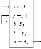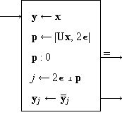
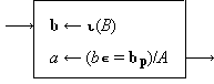
Program 4. A mapping specified by the permutation p

Program 4 describes a mapping from the argument b∊B to the function a∊A prescribed by the vector p. The process consists of three steps, the ranking of b in B, the permutation of the index j by p, and the selection of the correspondent A _pi. Since any set can be considered as a vector, the process can be expressed more concisely in terms of vector operations as shown in Program 5.

Program 5. Program 4 re-expressed in terms of vectors

The expression ⍳(B) denotes the identification vector of the set B, defined as the set considered as a vector, i.e.

      b ← ⍳(B)   ↔   b _i = B _i

A matrix whose rows and columns are all permutation vectors will be called a permutation matrix.^[d] A permutation matrix can clearly represent the operations in an abstract group. The group is Abelian if and only if the matrix is symmetric.
 

Files

A vector is frequently represented (stored) in a serial-access file in which the components are made available only in their natural sequence. To describe algorithms upon vectors so represented, it is convenient to introduce special notation for a file as follows. A file Φ of length n is a representation of a vector x of dimension n arranged as follows:

      λ(1), x₁, λ(2), x₂, …, λ(n), x _n, λ(n + 1)

The operation of transferring a component from a file to specify a quantity y is called reading the file and is denoted by y ← Φ. The transfer is terminated by the occurrence of a partition symbol, and if this symbol is λ(j) the file is then said to be in position j. A file may either be read forward (denoted by ₀Φ) or backward (denoted by ₁Φ). If a file originally in position j is read forward it transfers the component x _j and stops in position (j + 1),  j ε {(1, n)}. A file read backward from position j + 1 transfers the component x _j and stops in position j,  j ε {(1, n)}.

The position of a file Φ will be denoted by π(Φ). Thus the statement y ← π(Φ) specifies y as the position of Φ, whereas π(Φ) ← z positions the file to z. In particular, π(Φ) ← 1 denotes the rewinding of the file, and either π(Φ) ← (n + 1) or (using contracurrent indexing on the (n + 1) positions) π(Φ) ← –1 denote positioning to the end of the file. Any file for which the general positioning operation π(Φ) ← z is to be avoided as impossible or inefficient is called a serial or serial-access file.

A file may be produced by a sequence of recording statements, either forward:

      ₀Φ ← x _i,     i = 1, 2, …, n

      ₁Φ ← x _i,     i = n, n – 1, …, 1

As in reading, each forward (backward) record operation increments (decrements) the position of the file by one. A file which is only recorded during a process is called an output file of the process; a file which is only read is called an input file.

Each partition symbol may assume one of several values, λ₀, λ₁, …, λ _p, the partitions with larger indices demarking larger subgroups within the file. Thus if each component x _j were itself a vector y ^j (i.e. x is a matrix), then the last component of each y ^j might be followed by the partition λ₁, while the remaining components would each be followed by λ₀. The last component of the entire array might be followed by a partition λ₂. In recording an item, the associated partition is indicated by listing it after the item (e.g. Φ ← y, λ₂), except that the partition λ₀ is usually elided. The indicated partition then follows or precedes the associated item in the file according as the recording is forward or backward.

The indication provided by the distinct partition symbols is used to control an immediate (p + 1)-way branch in the program following each read operation. The branch is determined by the partition symbol which terminates the read.

Different files occurring in a process will be distinguished by righthand subscripts and superscripts, the latter being generally reserved to denote major classes of files (e.g. input and output). An array of files is therefore indexed like a matrix and the notation for compression may be applied to specify subsets of the array.

File notation is particularly useful in the description of sorting algorithms and of algorithms employing so-called “pushdown stores”.
 

The author is indebted to Dr. F.P. Brooks, Jr. for many important suggestions.
 

Notes

Discussion

R.A. FAIRTHORNE: There can be no very profitable discussion of new notations until they have been applied for some time by different people to different jobs. Always the inventor and his critics overlook some essential considerations.

On another aspect, I suggest that the author and others try to find better names for some of the operations, whatever the notations may be. In particular, “row (column) compression” implies that all elements remain in altered form, whereas in fact some are abstracted. Instead I would suggest “removal”, “omission”, “abbreviation”, “curtailment”, or “retention”, and for the inverse operation “insertion”, “augmentation”, “inflation”, according to whether the original part is referred to, or the parts that are added or removed. The final choice, whatever the term, must depend both on intrinsic descriptive merit and on harmony with other terms.

J. SHEKEL: In cases where vectors and matrices are distinguished from scalars by colour ^* or font, I suggest that special “zero” and ”equality” symbols should be used. This will enable some kind of “dimensional” check on the formulas and equations.

Incidentally, the line

      (x ≠ y) = xΔy

that was on the blackboard at the meeting illustrates the use of the same “equals” sign for two different meanings. Since you are constructing a new symbolism anyway, it would be better to avoid such ambiguities from the start.

I would propose the word “sifting” for the compress operation u/x. The operator u could then be called a “sieve”.

Concerning floors and ceilings, a general word of caution may be given against too much reliance on mnemonic techniques. Take the well known rhyme:

      Thirty days hath September, etc.

It seems that the words that rhyme are not the words that count, and vice versa …

K.E. IVERSON in reply: The notation has (as remarked in the oral presentation) been applied to a variety of jobs by a number of different people. These include language translation (A.G. Oettinger), machine organization (F.P. Brooks, Jr.), switching theory (P. Calingaert), and sorting theory and operations research (K.E. Iverson).

Concerning the nomenclature, I agree that the connotations of the word “compression” do not fit the case exactly. However, I find it preferable to the words suggested by Mr. Fairthorne (and to other alternatives which I have considered). For example, the terms “row removal” and “row omission” would imply deletion of an entire row of a matrix and would therefore not conform to the usage whereby the qualifier “row” indicates an operation upon a row of a matrix. The word “abbreviation” connotes no loss of information, and the word “curtail” connotes deletion of a tail or suffix only, both contrary to the intended meaning of the general compress operation u/x.

Answering Dr. Shekel, I must stress that none of the special vectors (such as ∊ ^j, ⍺ ^j, ⍵ ^j, ∊) contain a specification of dimension. As remarked in the oral presentation, this is a decided convenience, since in most cases the required dimension is implied by compatibility with associated operands. Where necessary, dimension can be specified by compression by a suitable prefix vector. For example, the factorial may be defined by the expression

      n! = ×/(⍺ⁿ/⍳) + (n = 0).

The zero symbol used for vectors as well as scalars can, if desired, be replaced by the zero vector , although I see no resulting gain in clarity.

The sign of equality is indeed used in two distinct senses, but the second occurs only in exposition, never in an algorithm.

On your second point the word “sifting” suggested for “compression” seems to possess no companion suitable for the converse operation of expansion.

As regards your third question — yes, moderation in all things. The caution seems somewhat gratuitous, however, since none of the mnemonic devices used appeal to anything so indirect and cumbersome as a rhyme.

* Used in the original typescripts; to indicate bold face —Ed.
 

Originally appeared in the Proceedings of a Conference on Information Theory, C. Cherry and W. Jackson, Editors, Imperial College, London, 1960-08-29. Images of the pages of the paper are available from here and here.