Recreational APL
Eugene McDonnell
June 1978
The Caret and the Stick Functions
| The power of using logical expressions as arithmetic operands is very great, as has been shown by Iverson. | |||
| — | George Radin and Paul Rogoway, “NPL: Highlights of a New Programming Language”, CACM 8, 1965 | ||
| But voluntarie signes, it is inoughe to knowe that this thei doe signifie. And if any manne can divise other, more easie or apter in use, that maie well be received. | |||
| — | Robert Recorde, The Whetstone of Witte, 1557 | ||
In a postscript to an earlier paper of mine
[1],
I very briefly covered a topic of some recreational significance,
namely “the whirling caret”.
In the present article, I give a more extended treatment
of the same subject, which is the design and use
of the relational and Boolean function symbols used in APL.
History
Of the relational and Boolean function symbols in APL, the first used was the equal sign (=), which was introduced by the Englishman Robert Recorde (1510-1558) in 1557 [2]. Recorde writes:
| And to avoide the tedioufe repetition of thefe woordes : is equalle to : I will fette as I doe often in woorke ufe, a paire of paralleles, or Gemowe (i.e., twin) lines of one lengthe, thus: == , bicaufe noe.2. thynges, can be moare equalle. |
There is some speculation that he was adapting to a mathematical context a symbol used by medieval scribes to indicate “est” (the Latin “is”). There is also some evidence that this sign was also in use in Bologna to mean the same thing. In any event, the sign was intended to permit assertions to be made regarding the equality of two expressions. Its use as a symbol for a function with value 1 or 0 was formalized by Iverson, for whom it was a generalization of the Kronecker delta, written δjk , which had the value 0 if j and k were unequal, and 1 otherwise. Iverson also extended the idea to include all the relational functions, writing [3]:
| The relational statement (α R β) is a logical variable which is true (equal to 1) if and only if α stands in the relation R to β. |
The Englishman Thomas Harriot (1560-1621), the first surveyor of Virginia and North Carolina (when he accompanied Sir Walter Raleigh to America), invented the symbols < and > to mean “less than” and “greater than” [4]. These appeared in his Artis Analyticae Praxis, first printed in 1631.
The Swiss Leonhard Euler (1707-1783) seems to have been
the first to use the not-equal sign formed
by placing a slash through the equal sign (≠)
[4].
This is significant because it showed a way
of turning a symbol into its negative.
Euler employed the same device in forming the
signs  and
and  for “not greater than” and “not less than”
[4].
These are not the symbols used in APL,
but I believe they should be, because they clearly show
the relationship to the direct form of the function.
for “not greater than” and “not less than”
[4].
These are not the symbols used in APL,
but I believe they should be, because they clearly show
the relationship to the direct form of the function.
The symbols that are used in APL for these two functions,
namely ≤ and ≥ , were introduced
by the Frenchman Pierre Bouguer in 1734.
The form of the symbol used by Bouguer showed
both bars of the equal sign as
in  and
and  [4].
I do not know who introduced the single bar symbols.
[4].
I do not know who introduced the single bar symbols.
A long time elapsed between the introduction of the last relational symbol and the first logical symbol. Symbolic logicians, beginning with George Boole, had used a variety of notations to signify the functions they needed in their work. It was the English mathematicians Alfred North Whitehead and Bertrand Russell who, in 1909 introduced the signs ~ for “not” and ∨ for “or”. Quine [5] suggests that the tilde (~) was an abbreviation of the script letter “n” and that the vee (∨) was derived from the first letter of the Latin word for “or”, namely “vel”.
Whitehead and Russell used the dot (.) for “and”, in common with many other authors — the same dot they used for multiplication. In current symbolic logic, the symbol & is often used for “and” — perhaps because the symbol is available on many typewriters, and it is an abbreviation of the Latin “et”, meaning “and”. The symbol used in APL for “and” appears to have come into use in symbolic logic sometime after 1928, the date of the first printing of my latest reference [2]. The earliest use I can find of the inverted vee (∧) to denote the “and” function is in a paper by the Pole Alfred Tarski published in 1933 [6].
The last of the symbols we shall be concerned with are those
for the joint denial and alternative denial functions,
that is, the “nor” and “nand” functions.
These are quite important functions,
because either one of them can be used
as the building block for all the others (see Problems).
Quine [5]
used the symbol  for “nor” and said,
“the vertical mark in '' may be thought of
as having the same canceling effect upon the sign '∨' ;
it is like the vertical mark in the inequality sign '≠' of arithmetic.”
Quine was certainly going in the right direction,
although it seems clear that
the canceling mark need not have a vertical orientation.
for “nor” and said,
“the vertical mark in '' may be thought of
as having the same canceling effect upon the sign '∨' ;
it is like the vertical mark in the inequality sign '≠' of arithmetic.”
Quine was certainly going in the right direction,
although it seems clear that
the canceling mark need not have a vertical orientation.
The initial implementation of APL\360 did not have the nand and nor functions. I don’t have a record of when they were introduced, but it was probably sometime in 1967. Their introduction was suggested by Peter Calingaert, who was then at Science Research Associates in Chicago and is now at the University of North Carolina. Calingaert wanted them because they would complete the set of the nontrivial Boolean functions of two variables. We shall discuss the meaning of “nontrivial” later, but just now we can say that “nontrivial” is the same as “essentially dyadic” and not merely formally so. The APL design group at the IBM Thomas J. Watson Research Center in Yorktown Heights, New York, was receptive to the suggestion, for reasons which have best been stated by Falkoff and Iverson [7]:
| One view of simplicity might exclude as redundant those functions which are easily expressed in terms of others. For example, ... ∧/l may be written as ~∨/~l . From another viewpoint it is simpler to use a more complete or symmetric set of primitives, since one need not remember which of a pair is provided and how to express the other in terms of it. In APL, completeness has been favored. For example, symbols are provided for all of the non-trivial logical functions, although all are easily expressed in terms of a small subset of them. |
Calingaert’s comment when I asked him about this episode was,
“As I recall, the proposal was accepted without discussion”
[8].
In the APL design group there was some experimentation
with the symbols to be used for the functions.
It is interesting that the initial symbols
were ∧ and ∨ overstruck
with a minus sign (-) .
This choice was much like the one Euler made in
negating < and > .
Unfortunately, the particular geometries of the characters
on the APL printing element made these combinations unpleasant,
and so eventually the tilde was used in place of the minus sign,
and thus we had ⍱ and ⍲ .
Theory
The input to a Boolean function of n variables can be represented as a Boolean vector of n elements representing the values of the arguments for a particular execution of the function. Because the arguments can have only the values 0 or 1, there are 2*n possible sets of distinct argument values. For example, for a Boolean function of 0, 1, 2, or 3 variables, there are 1, 2, 4, or 8 possible sets of argument values, respectively. These are shown below:
|
The result of the function for each of these possible argument values can be represented by a Boolean vector of length 2*n (one element for each set of argument possibilities). The Boolean function is completely defined by this vector of function results, which is called the intrinsic vector [3] of the function. Since there are 2*2*n distinct intrinsic vectors, there are 2*2*n distinct functions of n variables.
Suppose that the intrinsic vector for a two-variable function is 0 1 1 1 ; this means that when the argument values are both 0, the result is 0; for any other combination of argument values, the result is 1. In fact, 0 1 1 1 is the intrinsic vector for the “or” function. The following table is adapted from one given in APL Language [9]:
|


The rows headed ⍺ ⍵ represent the four possible sets of arguments that a dyadic Boolean function can have. Each column of the table to the right is the intrinsic vector for one of the 16 dyadic Boolean functions. For the nontrivial functions, the corresponding APL function symbol is appended. Note, for example, that the column with elements 0 1 1 1 has ∨ appended to it.
The publication points out:
| ... any boolean expression of two arguments ⍺ and ⍵ can be replaced by a simple APL expression as follows: evaluate the expression for the four possible cases, locate the corresponding column in the table, then use the function symbol at the foot of the column, or, if none occurs, use ⍺ or ⍵ or ~⍺ or ~⍵ or 0 or 1 as appropriate. |
For example, suppose we
set a←0 0 1 1 and b←0 1 0 1
(this gives us in the corresponding elements
of a and b all pairs of arguments).
Then the result of the expression a<b≤a=b≥a>b≠a∨b∧a b
is 1 0 0 0 .
Looking in the table, we find that the column with
value 1 0 0 0
has
b
is 1 0 0 0 .
Looking in the table, we find that the column with
value 1 0 0 0
has  appended to it,
so it must be that the long expression is replaceable
by ab ,
and such is the case.
appended to it,
so it must be that the long expression is replaceable
by ab ,
and such is the case.
The ten dyadic functions we’ve been discussing
are called the nontrivial Boolean dyadic functions,
but there is a sense in which everything
connected with logic is trivial.
The medieval curriculum comprised the seven liberal arts.
These were classified into two groups.
The higher group contained the four subjects
of geometry, astronomy, arithmetic,
and music and was called the quadrivium.
The elementary group contained the three subjects
of grammar, logic, and rhetoric and was called (are you ready?)
the trivium, from whence comes the adjective trivial.
Now, at Last, for the Recreation Part
Now that we have the ten dyadic Boolean function symbols, the urge to classify arises and must be appeased. If you were asked to sort the symbols into two piles based on their geometry, how would you do it? The chances are good that some of you would put the symbols with a caret shape in one pile and those without a caret in the other, thus creating a caret pile and a stick pile.
You know from the history I’ve given you how arbitrary the association is that groups the caret functions together, however, it is possible to show more intrinsic groupings. Suppose you were asked to sort the symbols into two piles based on their intrinsic vectors. Again, I believe that some of you would consider the parity of the vector sums as a way of classification. Doing this, you would find that the even sums correspond to the trivial and stick functions, and that the odd sums correspond to all the caret functions.
Is that all? No, it isn’t. Consider further the behavior of each of the functions when used to scan a truth table. Observe the following figure:
|
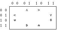 |
Observe that the caret symbol is rotated clockwise 90 degrees from box to box, going clockwise about the edges of the square, and that below the “equator”, the symbol is negated.
I won’t do any more than to say that the symbols for
the functions appear to have been chosen
with an aptitude bordering, like Cleveland, on eerie.
Problems
| 1a. |
The relational functions
are not the only non-Boolean functions that become Boolean
when their arguments are restricted to 0 and 1.
Multiplication, for example, is Boolean
(as George Boole showed in 1848
[10]).
What other non-Boolean scalar functions
become Boolean under this restriction of arguments?
| |||||||||||||||||||||||||||||||||
| b. |
It’s possible to define some Boolean functions
on an extended domain.
What extended definitions are suitable
for the functions in the table below?
| |||||||||||||||||||||||||||||||||
| 2a. |
As shown by Pierce (1880) and Sheffer (1913), the nor function can be used by itself to generate all 16 dyadic Boolean functions. Given a←0 0 1 1 and b←0 1 0 1 , for example, the intrinsic vector for the and function can be obtained by (a⍱a)⍱b⍱b . Provide the shortest expression possible for each intrinsic vector, 0 0 0 0 through 1 1 1 1 , using only the symbols a , b , ⍱ , ( , and ) and using ⍱ at least once. The shortest expressions known for each intrinsic vector (shown below evaluated in base 2) are the following:
| |||||||||||||||||||||||||||||||||
| b. |
Afterward, Sheffer also showed that the nand function can be used by itself to generate all 16 dyadic Boolean functions. Given the same a and b as in 2a., provide the shortest possible expression for each intrinsic vector (as in 2a.), but using only the symbols a , b , ⍲ , ( , and ) and using ⍲ at least once. The shortest expressions known for each intrinsic vector (again shown evaluated in base 2) are as follows:
| |||||||||||||||||||||||||||||||||
| 3. |
The stick function scans on Boolean arguments
are information preserving:
you can tell uniquely what the argument was if you see the result.
Furthermore, if you apply one of the stick scans often enough,
you will obtain your original argument.
How many times, in terms of ⍴v ,
does a stick function scan have to be applied, in general,
to a Boolean vector v in order to get v back again?
| |||||||||||||||||||||||||||||||||
| 4. | The “trivial” Boolean dyadic functions (for which APL provides no symbols) have some interesting properties. What is the number of distinct rows in the scans, using the trivial functions, of a truth table of order n ? |
References
| 1. | McDonnell, E.E. The caret functions. Proc. of the Sixth International APL User’s Conference, Anaheim, Calif., 1974. | |
| 2. | Cajori, F. A History of Mathematical Notations, Vol. I, Notation in Elementary Mathematics, Open Court, LaSalle, Ill., 1928. | |
| 3. | Iverson, K.E. A Programming Language. Wiley, New York, 1962. | |
| 4. | Ball, W.W.R. A Short Account of the History of Mathematics. Dover, New York, 1960. | |
| 5. | Quine, W.V.O. Mathematical Logic. Harper Torchbooks, New York, 1962. | |
| 6. | Tarski, A. Some observations on the concept of ⍵-consistency and ⍵-completeness. Translated from the original paper: Einige Betrachtungen über die Begriffe der ⍵-Widerspruchsfreiheit und der ⍵-Vollständigkeit, Monatshefte für Mathematik und Physik 40, (1933), 97-112. | |
| 7. | Falkoff, A.D., and Iverson, K.E. The design of APL. IBM Journal of Research and Development 17, (1973), 324-334. | |
| 8. | Calingaert, P. Private communication. | |
| 9. | APL Language. IBM Publication GC26-3847, Jan. 1976. | |
| 10. | Boole, G. An Investigation of the Laws of Thought. Dover, New York. | |
| 11. | McDonnell, E.E. A notation for the GCD and LCM functions. APL 75 Congress Proc. (Pisa), ACM, New York, 1975. |
Puzzle Solutions
(The following solutions refer to problems posed in the March 1978 issue of APL Quote Quad, pp. 43, 46-7.)
Page 43 — You were asked to write a function that prepares a table of all patterns of ⍺ 1’s and ⍵-⍺ 0’s, for ⍺≥0 and ⍵≥⍺ .
T.P. Holls of Poughkeepsie, New York, gives (in 0-origin):
f: ⍉(⍺=+⌿r)/r←(⍵⍴2)⊤⍳2*⍵
This is correct, but liable on many systems to use a large amount of space. The following doubly recursive function is more compact:
g: (0,⍺g⍵-1),[⎕io]1,(⍺-1)g⍵-1: ⍺∊0,⍵:(1,⍵)⍴⍺=⍵
Page 46
| 1. |
The inverse of 16807, mod 2147483647, is 1407677000.
| |
| 2. |
In APL\360 and its descendants, the technique for
computing ?n for n>2*31
uses two successive values of ⎕rl
to produce the desired result.
Thus, ?2*32 will advance ⎕rl by two steps.
| |
| 3. |
The “Petals Around the Rose” problem was solved by T.P. Holls (1-origin): a←(d-1)+.×2|d←?5⍴6 If you were unable to determine by inspection how to solve the problem, you might have done the following: assume the result is linearly related to the roll of the dice. Then, if m is the 16 by 5 matrix whose rows are the values of the dice as shown in the problem, and x is the vector of corresponding answers shown, the expression (1-origin) r←x⌹+/[2]m∘.=⍳6 gives a six-element vector result r , where r[i] is the value associated with the appearance of a die with i dots on it in the result. That is, we have solved an overdetermined linear system, a set of 16 simultaneous equations in 6 unknowns. The expression (⎕ct<|r)×r gives 0 0 2 0 4 0 showing that a die with a value of 3 is counted as 2,
and a die with a value of 5 is counted as 4.
You must figure out the significance of
the name “Petals Around the Rose” for yourself.
|
Correction —The answer given
for the cosine problem (page 48) should have
read ○/99⍴2 ,
not ∘/99⍴2 .
Supplement — Some additional entries were received for the “Puzzle of the Year, 1978”. Paul Penfield of MIT provided a solution for 54: ⌊*19-7+8 . Roger Hui of Edmonton, Alberta, provided seven better solutions:
17  6  19|-78
36  7  1⊥⍳97⌊8
38  7  19×⌈7⍟8
45  7  1⊥⍳9⌊78
54  8  1⌈9×7|-8
55  7  1⊥9-7↑8
92  8  1⊥9↑7+⍳8
and Alan Perlis of Yale also attacked 54,
coming up with 1⌈9×7-×8 .
Hui’s solution for 92 and all three solutions for 54 eliminated
the last 9-character solutions.
E. E. McDonnell
Palo Alto, California
First appeared in
APL Quote-Quad, Volume 8, Number 4, 1978-06.
The text requires the APL385 Unicode font, which can be
downloaded from
http://www.vector.org.uk/resource/apl385.ttf .
To resolve (or at least explain) problems with displaying
APL characters see
http://www.vector.org.uk/archive/display.htm .
last updated: 2009-08-26 17:00