SATN-40
Complex Numbers
Eugene McDonnell
Abstract
Complex numbers have been added to SHARP APL as an internal data type, and most of the primitive functions have been extended, where appropriate, to give complex results, and to take arrays containing complex numbers as arguments. Our implementation follows, in large measure, the design proposed by Paul Penfield, Jr., of MIT, in his ‘Proposal for a Complex APL’, given at the APL79 Conference.
Complex Number APL Available
| Once we conceive of the real line as embedded in a plane of complex numbers, we have entered a whole new domain of mathematics. All our old knowledge of real algebra and analysis becomes enlarged and enriched when reinterpreted in the complex domain. In addition, we immediately see countless new problems and questions which could not even have been raised in the context of the real numbers alone. | |
| Philip J. Davis and Reuben Hersh, The Mathematical Experience, Birkhausen, Boston, 1980 |
Complex numbers have been added to SHARP APL as an internal data type, and most of the primitive functions have been extended, where appropriate, to give complex results, and to take arrays containing complex numbers as arguments.
The extension is not complete. The floor, ceiling, residue, representation, and dyadic format functions have not been extended, because there remain points of uncertainty regarding their definitions. The way in which complex numbers are displayed in this release is provisional. As we gain more experience in the use of these numbers, we may change the form.
Until this announcement, writers of APL applications which required complex numbers had to simulate them by various devices which made the use of APL’s primitive functions and operators difficult. With this announcement, all the facilities of APL, except as noted in the preceding paragraph, may be used directly on complex numbers.
Generally speaking, existing applications
are not affected by this change.
The potential differences are local
to just a few primitive functions,
and are relatively minor.
Those functions which would benefit
from complex numbers yield complex results
instead of a domain error.
Complex constants and display
If two real scalar numeric constants are connected by the letter j , as in 3j¯4 , this is interpreted as the rectangular representation of a complex constant, with the real part first and the imaginary part second. Each of the two real numbers can be written using either decimal or scaled representations.
In displaying a column of numbers, some of which have nonzero imaginary parts, all the numbers in the column are right justified. For example, if z is the vector whose elements are the fifth roots of ¯32 , a one-column matrix w derived from it would be displayed as follows (with ⎕pp at 6):
      ⎕←w←5 1⍴z
  1.61803j1.17557
 ¯0.61803j1.90211
               ¯2
¯0.61803j¯1.90211
 1.61803j¯1.17557
The extensions of the primitive functions
Many of the primitive functions need no discussion since their extension to complex arguments is well understood. Here we shall describe only those functions whose extension is not obvious.
Conjugate: +⍵ is the conjugate of ⍵ , that is, the value obtained by reflecting ⍵ on the real axis. The conjugate of a real number ⍵ is equal to ⍵ . Thus a test to see if a number is real is ⍵=+⍵ .
Figure 1 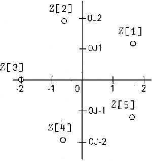
The elements of the vector z d are shown in Figure 1. The numbers z[1] and z[5] are conjugates, as are z[2] and z[4] . The number z[3] is equal to its own conjugate, since it is real.
Magnitude: |⍵ is the magnitude, or modulus as it is often called, of ⍵ . It is the value obtained by rotating ⍵ about the origin onto the positive axis. It may be defined as (⍵×+⍵)*0.5 . For example:
      |3j¯4               ←→   5
      |0.6j¯0.8           ←→   1
      |1.61803j¯1.17557   ←→   2
      |¯1j1               ←→   1.41421
Direction: ×⍵ is the direction of ⍵ , and is an extension of the signum function on real numbers. The direction of 0 is 0 . For nonzero ⍵ , ×⍵ is the value at the intersection with the unit circle of the ray from the origin through ⍵ . The magnitude of ×⍵ for nonzero ⍵ is 1 , and ×⍵ may be defined as ⍵÷|⍵ . For example:
      ×3j¯4               ←→   0.6j¯0.8
      ×0.03j¯0.04         ←→   0.6j¯0.8
      ×0j10               ←→   0j1
New circular function left arguments: Ten new left arguments ⍺ have been provided for ⍺○⍵ , primarily for use with complex numbers.
The correspondence between left argument value and function is different from that given in [1]. The assignments described here preserve as much as possible the association between odd functions (real part, imaginary part) with odd left arguments (9 and 11), and even functions (magnitude) with even left arguments (10). They also eliminate the gap which the earlier scheme had left between 8 and 11.
| (-⍺)○⍵ | ⍺ | ⍺○⍵ |
| -8○⍵ | 8 | 0j1×⍵×(1+⍵*¯2)*0.5 |
| ⍵ | 9 | (⍵++⍵)÷2 real part of ⍵ |
| +⍵ | 10 | |⍵ magnitude, or modulus, of ⍵ |
| 0j1×⍵ | 11 | (⍵-+⍵)÷0j2 imaginary part of ⍵ |
| *0j1×⍵ | 12 | 11○⍟⍵ arc or phase angle of ⍵ |
Two of these, 8○⍵ and ¯8○⍵ , are new Pythagorean functions, based on the expression (¯1-⍵*2)*0.5 , but modified to allow for both signs of the square root. The value of this function on reals is never real, which is why it had not been among the APL primitives before. With it, the set of Pythagorean functions is complete.
The remaining new left arguments for ⍺○⍵ are used in forming and decomposing complex numbers, using the rectangular and the polar representations of these numbers.
A number ⍵ may be decomposed into its real and imaginary parts by ¯9 ¯11○⍵ . For example:
9 11○3j¯4 ←→ 3 ¯4
Conversely, a pair of real numbers oj representing the real and imaginary parts of a complex number may be formed into that number by ¯9 ¯11+.○⍵ . For example:
¯9 ¯11+.○3 ¯4 ←→ 3j¯4
A number ⍵ may be decomposed into its magnitude and arc by 10 12○⍵ . For example:
10 12○3j¯4 ←→ 5 ¯0.927295
The arc is given in radians and is always greater than minus pi radians and less than or equal to pi radians. A positive number has an arc of 0. A negative number has an arc of pi. The arc of 0 is defined to be 0. For example:
            12○w
      0.628319
      1.88496
      3.14159
     ¯1.88496
     ¯0.628319
If deg:(180×⍵))÷○1 ⍝ radians to degrees , we can display the values of 12○⍵ in degrees. For example:
            deg 12○w
        36
       108
       180
      ¯108
       ¯36
Conversely, a pair of real numbers ⍵ , representing the magnitude and arc of a complex number may be formed into that number by ¯10 ¯12×.○⍵ . For example:
¯10 ¯12×.○5 ¯0.927295 ←→ 3j¯4
Equals and not equals: Two complex numbers are considered equal if the one smaller in magnitude lies on or within a circle whose center is at the one with larger magnitude, and whose radius is equal to ⎕ct times the larger magnitude.
Greatest common divisor and least common multiple: A complex integer is one whose real and imaginary parts are integers.
If a and b are complex integers, there are four other complex integers with the property that they are the largest in magnitude of all the complex integers which divide both a and b . a∨b is that one of these which is in the first quadrant, or on the positive axis.
For example, 117j44 and ¯63j¯16 have as greatest divisors the following numbers:
3j¯4 4j3 ¯3j4 ¯4j¯3
Of these, 4j3 is given as the value of 117j44∨¯63j¯16 since it is the one in the first quadrant.
a∨b is defined for noninteger complex numbers as well:
1.17j0.44∨¯0.63j¯0.16 ←→ 0.04j0.03
The least common multiple of two complex numbers, ⍺^⍵ , is defined by (⍺×⍵)÷⍺∨⍵ . For example:
¯182j¯107^¯7j55 ←→ ¯75j¯289
The least common multiple function is also
defined on non-integral complex numbers.
Functions whose domain does not include complex numbers
Because the complex numbers are not ordered,
those functions which depend on ordering
are not extended to complex numbers.
They are the dyadic
functions ⍺<⍵ , ⍺≤⍵ , ⍺≥⍵ , ⍺>⍵ , ⍺⌊⍵ , ⍺⌈⍵ , ⍺⍋⍵ ,
and ⍺⍒⍵ ,
and the monadic functions ⍋⍵ and ⍒⍵ .
Functions with deferred extensions
Because we have not agreed on definitions for the functions ⌈⍵ , ⌊⍵ , ⍺|⍵ , and ⍺⊤⍵ , they have not been extended at this time.
The formatting functions ⍺⎕fmt⍵ and ⍺⍕⍵ will take complex arguments, but their definitions have not been extended to take note of the imaginary parts of these numbers. Thus they format only the real part. For example:
            'bi3' ⎕fmt 3j¯4 0j2 0.2 5.2
      3


      5

            0⍕3j¯4 0j2 0.2 5.2
      3 0 0 5
Differences which may affect existing applications
Users should be aware that with this release there are differences in Sharp APL even if complex numbers are not used as arguments. This section describes these differences in detail.
There are two kinds of differences. In the first kind, a function which used to signal a domain error for certain real arguments now has a value which is not in general a real number. The functions in this category are ⍟⍵ and ⍺⍟⍵ for negative arguments, ⍺*⍵ for negative ⍺ and certain ⍵ , and ⍺○⍵ for certain arguments. In the second kind, a function now has a different value for certain arguments. There are two cases of this: ⍺*⍵ for negative ⍺ and certain ⍵ , and ¯4○⍵ . All this is covered in detail below.
In the first case, it seems unlikely that a user program would be affected, since one doesn’t ordinarily write a program to cause a domain error to be signalled. However, since Sharp introduced automatic trapping of errors in 1979, it is possible that someone could have written a program in such a way that a domain error used to be signalled by an expression which now has a value. This would, of course, cause the program behavior to be different. We judge this to be low in probability, but nonetheless feel obliged to caution our users, so that they may recognize the situation if it should occur.
We monitored the system extensively to try to judge the impact of the second of these changes (those where a different value is given). Over a one month period in 1979 there were 439 cases of ⍺*⍵ with ⍺<0 and ⍵ not an integer. On investigation, almost all of these uses were by Sharp development people, doing tests. We consulted with the owners of the few remaining workspaces and cautioned them of the impending change. There were only 176 uses of ¯4○⍵ , for all arguments. This compares with 6,149,426 uses of 1○⍵ , for example. Thus in both of these cases where a change in value occurs, we see little risk that any programs will be affected.
First case — domain error replaced by value: There are four functions which are affected.
| 1. |
The monadic logarithm function used to signal a domain error for negative arguments. With complex numbers available we can use the compatible extended definition of logarithm for all numbers except 0 : ⍟⍵ ←→ (⍟|⍵)+0j1×12○⍵ This definition is compatible since for positive arguments,
which have arcs of zero, the second term of the sum disappears.
We can thus provide a logarithm for arbitrary nonzero complex numbers,
and in particular for negative numbers.
For a negative number, the imaginary part
of its logarithm will be equal to pi,
since the arc of a negative number is pi radians.
| |
| 2. |
The dyadic logarithm function ⍺⍟⍵ also used
to signal a domain error if either argument was negative.
Since we can now give a value
to the logarithm of a negative number,
we can use the definition of ⍺⍟⍵ as (⍟⍵)÷⍟⍺
to give a definition for dyadic logarithms
of arbitrary nonzero numbers to arbitrary nonzero base,
and in particular to negative numbers and/or to negative bases.
| |
| 3. |
The power function ⍺*⍵ used to signal a domain error
for a negative ⍺ and ⍵ close or equal
to a rational number having an even denominator.
With complex numbers, such exponents are now permitted,
and the result in general is not real.
For example, ¯1*0.5 is 0j1 .
| |
| 4a. |
The dyadic circle function ⍺○⍵
has had the domain of its left argument extended,
as described above, to include the new
values ¯12 ¯11 ¯10 ¯9 ¯8 8 9 10 11 12 .
An attempt to use any of these as a left argument
used to give a domain error.
These new left arguments are intended primarily
for use in forming and decomposing nonreal complex numbers,
but they are valid also for real right arguments.
| |
| 4b. |
Several of the functions determined by particular left arguments of ⍺○⍵ have had their domains extended to include more real arguments, as well as having been extended to complex numbers in general. These are ¯7 ¯6 ¯4 2 1 0○⍵ . ¯7○⍵ : Formerly ⍵ had to be strictly between ¯1 and 1 . Now all arguments are valid except ¯1 and 1 . ¯6○⍵ : Formerly ⍵ had to be greater than or equal to 1 . Now all values are permitted. ¯4○⍵ : Formerly ⍵ could not be strictly between ¯1 and 1 . Now only 0 is prohibited. ¯2 ¯1 0○⍵ : Formerly ⍵ had to be between ¯1 and 1 . Now all numbers are permitted. |
Second case — changes in value: There are two functions in this category.
| 1. |
The defining expression for the power function ⍺*⍵ is *⍵×⍟⍺ (a) but this could not be used hitherto for negative ⍺ since logarithms of negative numbers were not defined. Nonetheless an attempt was made to give an answer, if ⍵ was not close or equal to a rational number with an even denominator, by assuming that in that case the exponent had an odd denominator n , and thus had one of its n roots on the negative axis. Up until now we have chosen to give that particular one of the n roots as the value. For example, referring to Figure 1, the elements of z are approximations to the fifth roots of ¯32 . One of these, ¯2 , is a real number, and is in fact the value that used to be given for the expression ¯32*0.2 . However, now that complex numbers are available we can use the defining expression (a) in every case where ⍺ is not zero. This ensures that functions such as ¯32*⍵ are (except for branch cuts) continuous over their entire domain. For example, the value of ¯32*0.2 is now given as 1.61803j1.17557 . The desired continuity can be seen by noting the closeness of adjacent values in the following example:
      3 1⍴¯32*0.1999 0.2 0.2001
1.61784j1.17465
1.61803j1.17557
1.61823j1.17649
| |
| 2. |
The definition of the ¯4○⍵ function has been changed from (¯1+⍵*2)*0.5 to ⍵×(1-⍵*¯2)*0.5 . Effectively, this doesn’t change the function for positive arguments, but for negative arguments the value is now negative instead of positive. For example, the value of ¯4○2 ¯2 used to be 1.73205 1.73205 . With the new definition the value is 1.73205 ¯1.73205 . |
General
The amount of storage required for one complex value is sixteen bytes.
⎕pp affects the display of each part of a complex number separately. For example, with ⎕pp←3 , we have:
¯9 ¯11+.○ 1234 0.1234 ←→ 1.23e3j0.123
An array whose type is complex can be used
with a function which requires a Boolean, integer,
or real value as argument
if the complex array values are sufficiently close
to Boolean, integer, or real values, respectively.
The tolerance used in making this determination
is not affected by ⎕ct .
For example, 3j1e¯20 may be used
to index the third element of a vector,
or as left argument to replicate.
Acknowledgments
The complex number extension to APL has been discussed in the APL community for many years. Paul Penfield, Jr., of MIT, played a leading role in elucidating the design problems, and made a comprehensive proposal for complex APL in [1]. The Sharp complex APL extension follows this proposal in all details except for the numbering of the new left arguments to ⍺○⍵ and in output formatting. Professor Penfield also was kind enough to criticize our implementation in the course of its development. The implementation was designed and developed by Doug Forkes and Gene McDonnell.
This SATN benefitted from comments given by Arlene Azzarello,
Paul Berry, Caroline Colburn, Doug Forkes, Ken Iverson,
and Roland Pesch, of I.P. Sharp Associates.
Reference
| [1] | Penfield, Paul Jr., ‘Proposal for a complex APL’, APL79 Conference Proceedings, ACM, 1979, pp 47-53. |
Bibliography
Most high school algebra texts cover the definitions of addition, subtraction, multiplication, reciprocation, and division on complex numbers. A.M. Gleason’s Fundamentals of Abstract Analysis, Addison Wesley, 1966, in chapters 10 and 15 covers the construction of the complex number system and the definitions of the exponential, logarithm, power, and trigonometric functions on complex numbers. A more elementary discussion of much of the same material is given in chapter 8 of K.E. Iverson’s Elementary Analysis, APL Press, Palo Alto. In Milton Abramowitz and Irene Stegun’s Handbook of Mathematical Tables, Dover, N.Y., 1965, may be found definitions of many of the analytic functions on complex arguments. A detailed exposition of the algorithm behind the complex factorial and complex binomial functions may be found in Hirondo Kuki’s ‘Complex Gamma Function with Error Control’, CACM 15, 4, April 1972. The paper by Paul Penfield, Jr., on ‘Principal Values and Branch Cuts in Complex APL’, to appear in the proceedings of APL81, discusses in complete detail the choices for locations of all branch cuts, direction of continuity of the branch cuts, and values at the end of the branch cuts, for all the analytic functions requiring them. We are obliged to Professor Penfield for providing us with an early draft of this valuable paper.
Those interested in the discussion
regarding the extension of the floor, ceiling, residue,
and representation functions may read
E.E. McDonnell’s ‘Complex Floor’, APL Congress 73,
North Holland/American Elsevier, 1973,
for one set of definitions, and
D.L. Forkes, ‘Complex Floor Revisited’,
to appear in the proceedings of APL81, for a counter-proposal.
Erratum
| • |
In the Complex constants and display section, the display of the fifth roots of ¯32 should read:
      ⎕←w←5 1⍴z
   1.61803j1.17557
 ¯0.618034j1.90211
                ¯2
¯0.618034j¯1.90211
  1.61803j¯1.17557
|
First appeared as SHARP APL Technical Note 40, Complex Numbers, 1981-06-20.
| created: | 2009-11-08 23:05 |
| updated: | 2012-09-24 14:00 |