A Programming Language

Kenneth E. Iverson
Research Division, IBM Corporation
Yorktown Heights, New York

Abstract

The paper describes a succinct problem-oriented programming language. The language is broad in scope, having been developed for, and applied effectively in, such diverse areas as microprogramming, switching theory, operations research, information retrieval, sorting theory, structure of compilers, search procedures, and language translation. The language permits a high degree of useful formalism. It relies heavily on a systematic extension of a small set of basic operations to vectors, matrices, and trees, and on a family of flexible selection operations controlled by logical vectors. Illustrations are drawn from a variety of applications.
 

The programming language outlined [1] here has been designed for the succinct description of algorithms. The intended range of algorithms is broad; effective applications include microprogramming, switching theory, operations research, information retrieval, sorting theory, structure of compilers, search procedures, and language translation. The symbols used have been chosen so as to be concise and mnemonic, and their choice has not been restricted to the character sets provided in contemporary printers and computers. A high degree of formalism is provided.
 

Basic Operations

The language is based on a consistent unification and extension of existing mathematical notations, and upon a systematic extension of a small set of basic arithmetic and logical operations to vectors, matrices, and trees. The arithmetic operations include the four familiar arithmetic operations and the absolute value (denoted by the usual symbols) as well as the floor, ceiling, and residue functions denoted and defined as follows:

where ⌊x⌋, ⌈x⌉, m, n, and q are integers.

The logical operations and, or, and not are defined upon the logical variables 0 and 1 and are denoted by ∧, ∨, and an overbar. They are augmented by the relational statement (proposition) (x R y) defined as follows. If x and y are any entities (e.g., numerals, alphabetic literals, or logical variables) and R is any relation defined upon them, then (x R y) is equal to 1 or 0 according to whether the relation R does or does not hold between x and y. Thus (i = j) is the familiar Kronecker delta δ_ij, (u ≠ v) is the exclusive or function of the logical variables u and v, and

sgn x = (x > 0) – (x < 0)

is the familiar sign function, defined as +1, 0, or –1 according as x is strictly positive, zero, or strictly negative.
 

Vectors and Matrices

A vector is denoted by a bold italic lowercase letter (e.g., x), its i-th component by x_i, and its dimension by ν(x). A matrix is denoted by a bold italic uppercase letter (e.g., X), its i-th row by X ⁱ, its j-th column by X_j, its ij-th element by X_jⁱ, its row dimension (i.e., the common dimension of its row vectors) by ν(X), and its column dimension by μ(X).

All of the basic operations are extended component-by-component to vectors and matrices. Thus,

The symbol (n) will denote a logical vector of dimension n whose components are all unity, and (n) therefore denotes the zero vector. The dimension n will be elided whenever it is clear from context. The cyclic left shift of a vector x is called left rotation. It is denoted by k ↑ x and defined by the relation:

y = (k ↑ x)  ↔  yi = xj,

where j = 1 + ν(x) | (i + k – 1). Right rotation is denoted by k ↓ x and is defined analogously.
 

Reduction

For each basic binary operator , the -reduction of a vector x is denoted by /x and defined by

/x = (…((x1 x2) x3) … xν(x)).

Thus +/x is the sum, and ×/x is the product of all components of x. Moreover, if u = (1, 0, 1), then +/u = 2, +/ = 1, ∧/u = 0, and ∨/u = 1.

Reduction is extended to matrices row-by-row:

z = /X  ↔  zi = /X i,

and column-by-column:

z = //X  ↔  zi = /Xi,

the column reduction being distinguished by the double slash.

For example , if u = (u₁, u₂) is a logical vector of dimension two, then De Morgan’s law may be expressed as:

.

Moreover, this is the valid generalization of De Morgan’s law to a vector u of arbitrary dimension.

The reduction operation can be extended to any relation R by substituting R for in the formal definition above. The parentheses in the definition now signify relational statements as well as grouping, and thus the expression ≠/u denotes the application of the exclusive-or over all components of the logical vector u. For example, ≠/(1, 0, 1) = ((1 ≠ 0) ≠ 1) = (1 ≠ 1) = 0. Induction can be used to show that

≠/u = 2|+/u, and .

Hence, ≠/u  =  , a useful companion to De Morgan’s law.
 

Matrix Product

The conventional matrix product AB may be defined as:

(AB)ji = +/ (Ai × Bj).

Adopting the notation A B for this product makes explicit the roles of the basic operations + and ×, and suggests the following useful generalization:

A B = 1/ (Ai 2 Bj),

where ₁ and ₂ are any operators or relations with suitable domains.

Thus C = M X is an “incidence matrix” such that C_jⁱ = 1 if and only if M ⁱ and X_j agree in all components. If M is the memory of a binary computer (i.e., M is a logical matrix and row M ⁱ is the i-th word of memory), and if x is an “argument register”, then (treating x as a one column matrix)

s = M x

defines the sense vector s of an associative memory such that s_i = 1 if and only if word M ⁱ agrees with x.

As further examples, R = P Q gives the number of places in which a component of P ⁱ exceeds the corresponding component of Q_j, and K = P Q is a “covering matrix” which indicates which rows of P cover (exceed in every component) which rows of Q.

De Morgan’s law and the identity

≠/u  =

establish a duality with respect to negation between ∧ and ∨, and between ≠ and =. This duality is easily extended to matrices. For example,

.

 

Selection

The formation of a vector y from a vector x by deleting certain components of x will be denoted by

y  =  u/x,

where u is a logical vector (of dimension ν(x)) and x_i is deleted if and only if u_i = 0. Thus u/x and /x provide a disjoint decomposition of x, and (x>)/x is the vector of all strictly positive components of x.

The operation u/x is called compression and is extended to matrices by row and by column as follows:

	Z = u/X	↔	Z i = u/X i,
	Z = u//X	↔	Zi = u/Xi.

The familiar identity concerning partitioned matrices can now be generalized as follows:

X Y  =  (/X) (//Y) + (u/X) (u//Y)

Since the identity depends only on the associativity and commutativity of the operators + and ×, it holds also for all operators (and relations) possessing these properties. Moreover,

u/(X Y) = X (u/Y),

and

u//(X Y) = (u//X) Y.

To illustrate other uses of compression, consider a bank ledger L so arranged that Lⁱ represents the i-th account, and L₁, L₂, and L₃ represent the vector of names, of account numbers, and of balances, respectively. Then the preparation of a list P (in the same format) of all accounts having a balance less than 2 dollars is described by the statement:

P ← (L3 < 2∊)//L,

where the arrow denotes specification (in the sense of the symbol = in Fortran and the symbol := in Algol).

Three useful operations converse to compression are defined as follows:

Mesh:   z = \a, u, b\  ↔  /z = a;     u/z = b Mask:   z = /a, u, b/  ↔  /z = /a; u/z = u/b Expansion:   z = u\b  ↔  z = \, u, b\ .

	\a, u, b\  =  /\a, u, u\b/ ,
	/a, u, b/  =  \/a, u, u/b\ .

Special Vectors

In addition to the full vector ∊(n) already defined, it is convenient to define the prefix vector ⍺ ^j(n) as a logical vector of dimension n whose first j components are unity. The suffix vector ⍵ ^j(n) is defined analogously. An infix vector having i leading 0’s followed by j 1’s can be denoted by  i↓⍺ ^j. When used in compression operations, these special vectors are very useful in specifying fixed formats.
 

Mixed Base Value

If the components of the vector y specify the radices of a mixed base number system and if x is any numerical vector of the same dimension, then the value of x in that number system is called the base y value of x, is denoted by y⊥x, and is defined formally by

y⊥x  =  w x,

where w is the weighting vector defined by w_ν(w) = 1 and w_i–1 = w_i × y_i. For example, if y = (24, 60, 60) and if x = (1, 2, 5) is the elapsed time in hours, minutes, and seconds, then y⊥x = 3725 is the elapsed time in seconds.

The value of x in a decimal system is denoted by (10∊)⊥x, and in a binary system by either (2∊)⊥x, or ⊥x. Moreover, if y is any real number, then (y∊)⊥x denotes the polynomial in y with coefficients x.
 

Application to Microprogramming

To illustrate the use of the notation in describing the operation of a computer, consider the IBM 7090 with a memory M of dimension 2¹⁵×36, a command vector c of dimension 36 representing the instruction next to be executed, a sequence vector s of dimension 15 representing the instruction counter, and a 3×15 index matrix I representing the three index registers. The instruction fetch phase of operation (excluding the channel trap) can then be described as in Figure 1. 0-origin indexing will be used for all vectors and matrices.

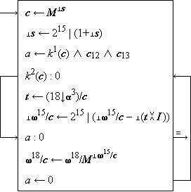
Instruction Fetch of IBM 7090
Figure 1

Step 1 shows the selection of the next instruction from the memory word specified by the instruction counter s and its transfer to the command register c. Step 2 shows the incrementation (reduced modulo 2¹⁵) of the counter s. The logical function k¹(c) of step 3 determines whether the instruction just fetched belongs to the class of instructions which are subject to indirect addressing, the bits c₁₂ and c₁₃ determine whether this particular instruction is to be indexed, and a is therefore set to unity only if indirect addressing is to be performed.

The function k²(c) determines whether the instruction is indexable. If k²(c) = 0, the branch from step 4 to step 7 skips the potential indexing of steps 5 and 6. As shown by step 6, indexing proceeds by oring together the index registers (i.e., rows of I) selected by the three tag bits t = (18↓⍺³)/c, subtracting the base two value of the resulting vector from the address portion of the instruction c, reducing the result modulo 2¹⁵, and respecifying the address portion of c accordingly.

The fetch terminates immediately from step 7 if no indirect addressing is indicated; otherwise step 8 performs the indirect addressing and the indexing phase is repeated. Step 9 limits the indirect addressing to a single level. It may be noted that all format information is presented directly in the microprogram.

The description of the execution phase of computer operation will be illustrated by the family of instructions for logical functions in the 7090. Representing the 38-bit accumulator by the logical vector u (with ν(u) = 38, and with u₀, u₁, and u₂ representing the sign, q, and p bits, respectively), these instructions may be described as in Figure 2.

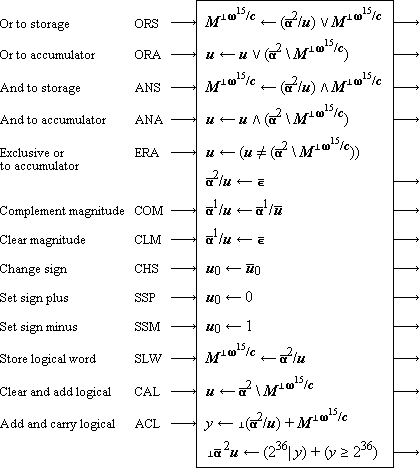
Instructions in IBM 7090
Figure 2
 

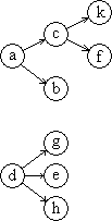
Ordered Trees

A tree can be represented graphically as in Figure 3(a) and, since it is a special case of a directed graph, it can also be represented by a node vector n and a connection matrix C as in Figure 3(b).

		n = ( a, c, f, k, e, d, h, g, b )   C = 0 1 0 0 0 0 0 0 1 0 0 1 1 0 0 0 0 0 0 0 0 0 0 0 0 0 0 0 0 0 0 0 0 0 0 0 0 0 0 0 0 0 0 0 0 0 0 0 0 1 0 1 1 0 0 0 0 0 0 0 0 0 0 0 0 0 0 0 0 0 0 0 0 0 0 0 0 0 0 0 0
Figure 3(a)		Figure 3(b)

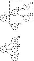
Defining an ordered tree as a tree in which the set of branches emanating from each node has a specific ordering, a simple indexing system for order trees can be defined in the manner indicated by Figure 4(a). The dimension of the vector index i assigned to each node is equal to the number of the level on which it occurs. If T is an ordered tree, then T_i will denote the subtree rooted in the node with index i. Thus T_(1,1) is the subtree enclosed in broken lines in Figure 4(a). Moreover, Tⁱ will denote the (unique) path vector comprising all nodes from the root to node i. Thus T^(1,2) = (a, b). The maximum dimension occurring among the index vectors is called the height of the tree and is denoted ν(T).

		d     n    I  2 2 0 0 0 3 0 0 0 a c k f b d g e h 1 0 0 1 1 0 1 1 1 1 1 2 1 2 0 2 0 0 2 1 0 2 2 0 2 3 0		d ′    n′   I &prime  2 3 2 0 0 0 0 0 0 a d c b g e h k f 0 0 1 0 0 2 0 1 1 0 1 2 0 2 1 0 2 2 0 2 3 1 1 1 1 1 2
T Figure 4(a)		[T Figure 4(b)		]T Figure 4(c)

The index vector notation proves very convenient in describing algorithms involving tree operands. Moreover, it provides a simple formalization of the two important respresentations of a tree, the Lukasiewicz representation and the level-by-level list.

If each index vector is augmented by sufficient null components (denoted by 0) to bring all to a common dimension equal to the height of the tree, then they may all be arrayed in an index matrix I as in Figure 4(b). If, as in Figure 4(b), the node vector n is defined such that n_j is the value of the node indicated by (the significant part of) the index vector I ^j, then the matrix obtained by appending n to I provides an unambiguous representation of the tree T. It is convenient to also append the degree vector d such that d_j is the degree (i.e., the number of branches emanating from) node I ^j. The resulting matrix of ν(T)+2 columns is called a full list matrix of T.

Any matrix obtained by interchanging rows of a full list matrix is also a full list matrix and is again an unequivocal representation of the tree. If, as in Figure 4(c), the index vectors are right justified and arranged in increasing order on their value as integers (in a positional number system), the resulting list matrix is called a full right list matrix and is denoted by ]T. If, as in Figure 4(b), the index vectors are left justified and arranged in increasing order as fractions, the list matrix is called a full left list matrix and is denoted by [T.

The right list groups nodes by levels, and the left list by subtrees. Moreover, in both cases the degree and node vector together (that is, ⍺²/(]T) or ⍺²/([T)) can be shown to provide an unequivocal representation of the tree without the index matrix. If,as in the case of a tree representing a compound statement involving operators of known degree, the degree vector d is a known function of the node vector n, then the tree may be represented by the node vector n alone. In the case of the left list, this leads to the Lukasiewicz^[a] notation for compound statements.
 

Applications of Tree Notation

The tree notation and the right and left list matrices are useful in many areas^[b]. These include sorting algorithms such as the repeated selection sort [4], the analysis of compound statements and their transformation to optimal form as required in a compiler, and the construction of an optimal variable-length code of the Huffman [5] prefix type. The sorting algorithm proceeds level by level and the right list representation of the tree is therefore most suitable. The analysis of a compound statement proceeds by subtrees and the left list (i.e., Lukasiewicz) form is therefore appropriate. The index vectors of the leaves of any tree clearly form a legitimate Huffman prefix code and the construction of such a code proceeds by combining subtrees in a manner dictated by the frequencies of the characters to be encoded, and therefore employs a left list. However, the characters are finally assigned in order of decreasing frequency to the leaves in right list order, and the index matrix produced must therefore be brought to right list order.
 

References

Notes