A Common Language
for Hardware, Software, and Applications

Kenneth E. Iverson

Thomas J. Watson Research Center, IBM
Yorktown Heights, New York
 

Introduction

Algorithms commonly used in automatic data processing are, when considered in terms of the sequence of individual physical operations actually executed, incredibly complex. Such algorithms are normally made amenable to human comprehension and analysis by expressing them in a more compact and abstract form which suppresses systematic detail. This suppression of detail commonly occurs in several fairly well defined stages, providing a hierarchy of distinct descriptions of the algorithm at different levels of detail. For example, an algorithm expressed in the FORTRAN language may be transformed by a compiler to a machine code description at a greater level of detail which is in turn transformed by the “hardware” of the computer into the detailed algorithm actually executed.

Distinct and independent languages have commonly been developed for the various levels used. For example, the operations and syntax of the FORTRAN language show little semblance to the operations and syntax of the computer code into which it is translated, and neither FORTRAN nor the machine language resemble the circuit diagrams and other descriptors of the processes eventually executed by the machine. There are, nevertheless, compelling reasons for attempting to use a single “universal” language applicable to all levels, or at least a single core language which may be slightly augmented in different ways at the various levels.

First, it is difficult, and perhaps undesirable, to make a precise separation into a small number of levels. For example, the programmer or analyst operating at the highest (least detailed) level, may find it convenient or necessary to revert to a lower level to attain greater efficiency in eventual execution or to employ convenient operations not available at the higher level. Programming languages such as FORTRAN commonly permit the use of lower levels, frequently of a lower level “assembly language” and of the underlying machine language. However, the employment of disparate languages on the various levels clearly complicates their use in this manner.

Second, it is not even possible to make a clear separation of level between the software (metaprograms which transform the higher level algorithms) and the hardware, since the hardware circuits may incorporate permanent or semipermanent memory which determines its action and hence the computer language. If this special memory can itself be changed by the execution of a program, its action may be considered that of software, but if the memory is “read-only” its action is that of hardware—leaving a rather tenuous distinction between software and hardware which is likely to be further blurred in the future.

Finally, in the design of a data processing system it is imperative to maintain close communication between the programmers (i.e., the ultimate users), the software designers, and the hardware designers, not to mention the communication required among the various groups within any one of these levels. In particular, it is desirable to be able to describe the metaprograms of the software and the microprograms of the hardware in a common language accessible to all.

The language presented in Reference 1 shows promise as a universal language, and the present paper is devoted to illustrating its use at a variety of levels, from microprograms, through metaprograms, to “applications” programs in a variety of areas. To keep the treatment within reasonable bounds, much of the illustration will be limited to reference to other published material. For the same reason the presentation of the language itself will be limited to a summary of that portion required for microprogramming (Table 1), augmented by brief definitions of further operations as required.
 

Microprograms

In the so-called “systems design” of a computer it is perhaps best to describe the computer at a level suited to the machine language programmer. This type of description has been explored in detail for a single machine (the IBM 7090) in Reference 1, and more briefly in Reference 2. Attention will therefore be restricted to problems of description on a more detailed level, to specialized equipment such as associative memory, and to the practical problem of keying and printing microprograms which arise from their use in design automation and simulation.

The need for extending the detail in a microprogram may arise from restrictions on the operations permitted (e.g., logical or and negation, but not and), from restrictions on the data paths provided, and from a need to specify the overall “control” circuits which (by controlling the data paths) determine the sequence in the microprogram, to name but a few. For example, the basic “instruction fetch“ operation of fetching from a memory (i.e., a logical matrix) M the word (i.e., row) M ⁱ selected according to the base two value of the instruction location register s (that is, i = ⊥s), and transferring it to the command register c, may be described as

c ← M⊥s.

Suppose, however, that the base two value operation (i.e., address decoding) is not provided on the register s directly, but only on a special register a to which s may be transferred. The fetch then becomes

a ← s c ← M⊥a.

Suppose, moreover, that all communication with memory must pass through a buffer register b, that each transfer out of a memory word M ⁱ is accompanied by a subsequent reset to zero of that word (that is, M ⁱ ← ), that every transfer from a register (or word of memory) x, to a register (or word of memory) y must be of the form

y ← x ∨ y,

and that any register may be reset to zero, then the instruction fetch becomes

1     a ← 2   a ← s ∨ a 3   b ← 4   b ← M⊥a ∨ b 5   M⊥a ← 6   M⊥a ← b ∨ M⊥a 7   c ← 8   c ← b ∨ c

In this final form, the successive statements correspond directly (except for the bracketed pair 4 and 5 which together comprise an indivisible operation) to individual register-to-register transfers. Each statement can, in fact, be taken as the “name” of the corresponding set of data gates, and the overall control circuits need only cycle through a set of states which activate the data gates in the sequence indicated.

The sequence indicated in a microprogram such as the above is more restrictive than necessary and certain of the statements (such as 1 and 3 or 6 and 7) could be executed concurrently without altering the overall result. Such overlapping is normally employed to increase the speed of execution of microprograms. The corresponding relaxation of sequence constraints complicates their specification, e.g., execution of statement k might be permitted to begin as soon as statements h, i and j were completed. Senzig (Reference 3) proposes some useful techniques and conventions for this purpose.

The “tag” portion of an associative memory can, as shown in Reference 2, be characterized as a memory M, an argument vector x, and a sense vector s related by the expression

s = M x

or by the equivalent expression

,

obtained by applying De Morgan’s law. Falkoff (Reference 4) has used microprograms of the type discussed here in a systematic exploration of schemes for the realization of associative memories for a variety of functions including exact match, largest tag, and nearest larger tag.

Because the symbols used in the language have been chosen for their mnemonic properties rather than for compatibility with the character sets of existing keyboards and printers, transliteration is required in entering microprograms into a computer, perhaps for processing by a simulation or design automation metaprogram. For that portion of the language which is required in microprogramming, Reference 5 provides a simple and mnemonic solution of the transliteration problem. It is based upon a two-character representation of each symbol in which the second character need be specified but rarely. Moreover, it provides a simple representation of the index structure (permitting subscripts and superscripts to an arbitrary number of levels) based upon a Lukasiewicz or parenthesis-free representation of the corresponding tree.
 

Metaprograms

Just as a microprogram description of a computer (couched at a suitable level) can provide a clear specification of the corresponding computer language, so can a program description of a compiler or other metaprogram give a clear specification of the “macro-language” which it accepts as input. No complete description of a compiler expressed in the present language has been published, but several aspects have been treated. Brooks and Iverson (Chapter 8, Reference 6) treat the SOAP assembler in some detail, particularly the use of the open addressing system and “availability” indicators in the construction and use of symbol tables, and also treat the problem of generators. Reference 1 treats the analysis of compound statements in compilers, including the optimization of a parenthesis-free statement and the translations between parenthesis and parenthesis-free forms. The latter has also been treated (using an emasculated form of the language) by Oettinger (Reference 7) and by Huzino (Reference 8); it will also be used for illustration here.

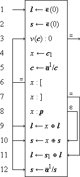
Consider a vector c representing a compound statement in complete^[a] parenthesis form employing operators drawn from a set p (e.g., p = (+, ×, –, ÷)). Then Program 1 shows an algorithm for translating any well-formed statement c into the equivalent statement l in parenthesis-free (i.e., Lukasiewicz) form.

Program 1
Translation from complete parenthesis statement c
to equivalent Lukasiewicz statement l

Program 1 - The components of c are examined, and deleted from c, in order from left to right (steps 4, 5). According to the decisions on steps 6, 7, and 8,^[b] each component is discarded if it is a left parenthesis, appended at the head of the resulting vector l if it is a variable (step 9), appended at the head of the auxiliary stack vector s if it is an operator (step 10), and initiates a transfer of the leading component of the stack s to the head of the result l if it is a right parenthesis (steps 11, 12). The behavior is perhaps best appreciated by tracing the program for a given case, e.g., if c = ([, [, x, +, y, ], ×, [, p, +, q, ],]), then l = (×, +, q, p, +, y, x).
 

Applications

Areas in which the programming language has been applied include search and sorting procedures, symbolic logic, linear programming, information retrieval, and music theory. The first two are treated extensively in Reference 1, and Reference 9 illustrates the application to linear programming by a 13-step algorithm for the simplex method. The areas of symbolic logic and matrix algebra illustrate particularly the utility of the formalism provided. Salton (Reference 10) has treated some aspects of information retrieval, making particular use of the notation for trees. Kassler’s use in music concerns the analysis of Schoenberg’s 12-tone system of composition (Reference 11).

Three applications will be illustrated here: search procedures, the relations among the canonical forms of symbolic logic, and matrix inversion.

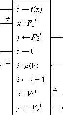
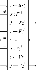
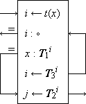
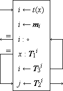
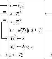
Search Algorithms. Figure 1 shows search programs and examples (taken from Reference 1) for five methods of “hash addressing” (cf. Peterson, Reference 12), wherein the functional correspondent of an argument x is determined by using some key transformation function t which maps each argument x into an integer i in the range of the indices of some table (i.e., matrix) which contains the arguments and their correspondents. The key transformation t is, in general, a many-to-one function and the index i is merely used as the starting point in searching the table for the given argument x. Figure 1 is otherwise self-explanatory. Method (e) is the widely used open addressing system described by Peterson (Reference 12).

Symbolic Logic. If x is a logical vector and T is a logical matrix of dimension 2^ν(x) × ν(x) such that the base two value of T ⁱ is i (that is, ⊥T = ⍳⁰(2^ν(x))), then the rows of T define the domain of the argument x, and any logical function f(x) defined on x can be completely specified by the intrinsic vector i(f) such that i_j(f) = f(T ^j).

Expansion of the expression p = T x shows that p is the vector of minterms in x, and consequently

	f(x)	=  γ(f,∨) p
		=  γ(f,∨) (T x),

where γ(f,∨) denotes the characteristic vector of the function f in the disjunctive canonical form. Formally, γ(f,∨) may be defined by the relation

i(f)  =  γ(f,∨) (T ),

(1)

where denotes the transpose of . It is easily shown that T is equal to the identity matrix, and hence that γ(f,∨) = i(f).

In a similar manner, the expression for the exclusive disjunctive canonical form may be written (Reference 1, Chapter 7) as

i(f)  =  γ(f,≠) (T ),

(2)

and the relation between the intrinsic vector and the exclusive disjunctive characteristic vector γ(f,≠) (first derived by Muller, Reference 13) is given directly by the square matrix S = T . The properties of the matrix S are easily derived from this formulation. Moreover, the formal application of De Morgan’s laws to equations (1) and (2) yields the two remaining canonical forms directly (Reference 1, Chapter 7).

Matrix Inversion. The method of matrix inversion using Gauss-Jordan (complete) elimination with pivoting and restricting the total major storage to a single square matrix augmented by one column (described in Reference 14 and 15) involves enough selection, permutation, and decision type operations to render its complete description by classical matrix notation rather awkward. Program 2 describes the entire process. The starred statements perform the pivoting operations and their omission leaves a valid program without pivoting; exegesis of the program will first be limited to the abbreviated program without pivoting.

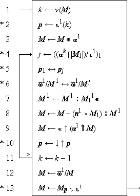Program 2
Matrix inversion by Gauss-Jordan elimination

Program 2 - Step 1 initializes the counter k which limits (step 11) the number of iterations and step 3 appends to the given square matrix M a final column of the form (1, 0, 0, …, 0) which is excised (step 12) only after completion of the main inversion process. Step 7 divides the pivot (i.e., the first) row by the pivot element, and step 8 subtracts from M the outer product of its first row (except that the first element is replaced by zero) with its first column.^[c] The result of steps 7 and 8 is to reduce the first column of M to the form (1, 0, 0, …, 0) as required in Jordan elimination.

The net result of step 9 is to bring the next pivot row to first position and the next pivot element to first position within it by (1) cycling the old pivot row to last place and the remaining rows up by one place, and (2) cycling the leading column (1, 0, 0, …, 0) to last place (thus restoring the configuration produced by step 3) and the remaining columns one place to the left. The column rotation^{[d] 1} M rotates all columns save the first upward by one place, and the subsequent row rotation ∊↑ rotates all rows to the left by one place.

The pivoting provided by steps 2, 4, 5, 6, 10, and 13 proceeds as follows. Step 4 determines the index j of the next pivot row by selecting the maximum^[e] over the magnitudes of the first k elements of the first column, where k = ν(M) + 1 – q on the q-th iteration. Step 6 interchanges the first row with the selected pivot row, except for their final components. Step 5 records the interchange in the permutation vector^[f] p which is itself initialized (step 2) to the value of the identity permutation vector ⍳¹(k) = (1, 2, … , k). The rotation of p on step 10 is necessitated by the corresponding rotations of the matrix M (which it indexes) on step 9. Step 13 performs the appropriate inverse reordering^[g] among the columns of the resulting inverse M.

A description in the ALGOL language of matrix inversion by the Gauss-Jordan method is provided in Reference 16.
 

References

Notes

a.		In complete parenthesis form all implied parentheses are explicity included, e.g., the statement ((x + y) × (p + q)) is represented by c = ([, [, x, +, y, ], ×, [, p, +, q, ], ]).
b.		A branch is followed if the relation with which it is labelled holds between the quantities separated by the colon. The relation “ε” denotes set membership.
c.		The outer product Z of vector x by vector y is the “column by row product” denoted by Z ← x y and defined by Zji = xi × yj.
d.		The row rotation k ↑ X is a row-by-row extension of the rotation k ↑ x, that is, (k ↑ X)i = ki ↑ X i. Similarly, (k X)j = kj ↑ X j.
e.		The expression u = v ⌈ x denotes a logical vector u such that ui = 1 if and only if xi is a maximum among those components xk such that vk = 1. Clearly, u/⍳1 is the vector of indices of the (restricted) maxima, and (u/⍳1)1 is the first among them.
f.		A permutation vector is any vector p whose components take on all the values 1, 2, …, ν(p). The expression y = xp denotes that y is a permutation of x defined by yi = xpi.
g.		Permutation is extended to matrices as follows:   N = Mp  ↔  Nj = Mpj ,   L = M p  ↔  Li = M pi. The expression a ⍳ x is called the a index of x and is defined by the relation a ⍳ x = j, where x = aj. If x is a vector, then j = a ⍳ x is defined by ji = a ⍳ xi. Consequently, p ⍳ ⍳1 denotes the permutation inverse to p.

Figure 1. Programs and examples for methods of scanning
equivalence classes defined by a 1-origin key transformation t

Data of examples
 

1     F = Friday   6 2 Sunday   1 3 Tuesday   3 4 ∘   ∘ 5 ∘   ∘ 6 Wesnesday   4   1     V = Monday   2 2 Thursday   5 3 Saturday   7

(a) Overflow
 

1     F = Friday   6   ∘ 2 Sunday   1   1 3 Tuesday   3   2 4 ∘   ∘   ∘ 5 ∘   ∘   ∘ 6 Wesnesday   4   ∘   1     V = Monday   2   3 2 Thursday   5   ∘ 3 Saturday   7   ∘

(b) Overflow with chaining
 

1     T = Friday   6   ∘ 2 Sunday   1   4 3 Tuesday   3   5 4 Monday   2   7 5 Thursday   5   ∘ 6 Wesnesday   4   ∘ 7 Saturday   7   ∘

(c) Single table with chaining
 

1     T = Sunday   1   2 2 Monday   2   7 3 Tuesday   3   5 4 Wednesday   4   ∘ 5 Thursday   5   ∘ 6 Friday   6   ∘ 7 Saturday   7   ∘       m = (6, 1, 3, ∘, ∘, 4)

(d) Single table with chaining and mapping vector
 

1     T = Friday   6 2 Sunday   1 3 Monday   2 4 Tuesday   3 5 Thursday   5 6 Wednesday   4 7 Saturday   7

(e) Open addressing system-construction and use of table