|
To My Many Teachers
Preface
Applied mathematics is largely concerned with the design and analysis of explicit procedures for calculating the exact or approximate values of various functions. Such explicit procedures are called algorithms or programs. Because an effective notation for the description of programs exhibits considerable syntactic structure, it is called a programming language.
Much of applied mathematics, particularly the more recent computer-related areas which cut across the older disciplines, suffers from the lack of an adequate programming language. It is the central thesis of this book that the descriptive and analytic power of an adequate programming language amply repays the considerable effort required for its mastery. This thesis is developed by first presenting the entire language and then applying it in later chapters to several major topics.
The areas of application are chosen primarily for their intrinsic interest and lack of previous treatment, but they are also designed to illustrate the universality and other facets of the language. For example, the microprogramming of Chapter 2 illustrates the divisibility of the language, i.e., the ability to treat a restricted area using only a small portion of the complete language. Chapter 6 (Sorting) shows its capacity to compass a relatively complex and detailed topic in a short space. Chapter 7 (The Logical Calculus) emphasizes the formal manipulability of the language and its utility in theoretical work.
The material was developed largely in a graduate course given for several years at Harvard and in a later course presented repeatedly at the IBM Systems Research Institute in New York. It should prove suitable for a two-semester course at the senior or graduate level. Although for certain audiences an initial presentation of the entire language may be appropriate, I have found it helpful to motivate the development by presenting the minimum notation required for a given topic, proceeding to its treatment (e.g., microprogramming), and then returning to further notation. The 130-odd problems not only provide the necessary finger exercises but also develop results of general interest.
Chapter 1 or some part of it is prerequisite to each of the remaining “applications” chapters, but the applications chapters are virtually independent of one another. A complete appreciation of search techniques (Chapter 4) does, however, require a knowledge of methods of representation (Chapter 3). The cross references which do occur in the applications chapters are either nonessential or are specific to a given figure, table, or program. The entire language presented in Chapter 1 is summarized for reference at the end of the book.
In any work spanning several years it is impossible to acknowledge adequately the many contributions made by others. Two major acknowledgments are in order: the first to Professor Howard Aiken, Director Emeritus of the Harvard Computation Laboratory, and the second to Dr. F.P. Brooks, Jr. now of IBM.
It was Professor Aiken who first guided me into this work and who provided support and encouragement in the early years when it mattered. The unusually large contribution by Dr. Brooks arose as follows. Several chapters of the present work were originally prepared for inclusion in a joint work which eventually passed the bounds of a single book and evolved into our joint Automatic Data Processing and the present volume. Before the split, several drafts of these chapters had received careful review at the hands of Dr. Brooks, reviews which contributed many valuable ideas on organization, presentation, and direction of investigation, as well as numerous specific suggestions.
The contributions of the 200-odd students who suffered through the development of the material must perforce be acknowledged collectively, as must the contributions of many of my colleagues at the Harvard Computation Laboratory. To Professor G.A. Salton and Dr. W.L. Eastman, I am indebted for careful reading of drafts of various sections and for comments arising from their use of some of the material in courses. Dr. Eastman, in particular, exorcised many subtle errors from the sorting programs of Chapter 6. To Professor A.G. Oettinger and his students I am indebted for many helpful discussions arising out of his early use of the notation. My debt to Professor R.L. Ashenhurst, now of the University of Chicago, is apparent from the references to his early (and unfortunately unpublished) work in sorting.
Of my colleagues at the IBM Research Center, Messrs. L.R. Johnson and A.D. Falkoff, and Dr. H. Hellerman have, through their own use of the notation, contributed many helpful suggestions. I am particularly indebted to L.R. Johnson for many fruitful discussions on the applications of trees, and for his unfailing support.
On the technical side, I have enjoyed the assistance of unusually competent typists and draughtsmen, chief among them being Mrs. Arthur Aulenback, Mrs. Philip J. Seaward, Jr., Mrs. Paul Bushek, Miss J.L. Hegeman, and Messrs. William Minty and Robert Burns. Miss Jacquelin Sanborn provided much early and continuing guidance in matters of style, format, and typography. I am indebted to my wife for assistance in preparing the final draft.
| Kenneth E. Iverson |
| May, 1962 |
| Mount Kisco, New York |
Chapter 1 The Language
1.1 Introduction
Applied mathematics is concerned with the design and analysis of algorithms or programs. The systematic treatment of complex algorithms requires a suitable programming language for their description, and such a programming language should be concise, precise, consistent over a wide area of application, mnemonic, and economical of symbols; it should exhibit clearly the constraints on the sequence in which operations are performed; and it should permit the description of a process to be independent of the particular representation chosen for the data.
Existing languages prove unsuitable for a variety of reasons. Computer coding specifies sequence constraints adequately and is also comprehensive, since the logical functions provided by the branch instructions can, in principle, be employed to synthesize any finite algorithm. However, the set of basic operations provided is not, in general, directly suited to the execution of commonly needed processes, and the numeric symbols used for variables have little mnemonic value. Moreover, the description provided by computer coding depends directly on the particular representation chosen for the data, and it therefore cannot serve as a description of the algorithm per se.
Ordinary English lacks both precision and conciseness. The widely used Goldstine-von Neumann (1947) flowcharting provides the conciseness necessary to an over-all view of the processes, only at the cost of suppressing essential detail. The so-called pseudo-English used as a basis for certain automatic programming systems suffers from the same defect. Moreover, the potential mnemonic advantage in substituting familiar English words and phrases for less familiar but more compact mathematical symbols fails to materialize because of the obvious but unwonted precision required in their use.
Most of the concepts and operations needed
in a programming language have already been defined
and developed in one or another branch of mathematics.
Therefore, much use can and will be made
of existing notations.
However, since most notations are specialized
to a narrow field of discourse,
a consistent unification must be provided.
For example, separate and conflicting notations
have been developed for the treatment of sets,
logical variables, vectors, matrices, and trees,
all of which may, in the broad universe of discourse
of data processing, occur in a single algorithm.
1.2 Programs
A program statement is the specification of some quantity or quantities in terms of some finite operation upon specified operands. Specification is symbolized by an arrow directed toward the specified quantity. thus “y is specified by sin x” is a statement denoted by
y ← sin x.
A set of statements together with a specified order of execution constitutes a program. The program is finite if the number of executions is finite. The results of the program are some subset of the quantities specified by the program. The sequence or order of execution will be defined by the order of listing and otherwise by arrows connecting any statement to its successor. A cyclic sequence of statements is called a loop.
 | |||
| Program 1.1 Finite Program | Program 1.2 Infinite Program |
Thus Program 1.1 is a program of two statements defining the result v as the (approximate) area of a circle of radius x, whereas Program 1.2 is an infinite program in which the quantity z is specified as (2y)n on the nth execution of the two statement loop. Statements will be numbered on the left for reference.
A number of similar programs may be subsumed under a single more general program as follows. At certain branch points in the program a finite number of alternative statements are specified as possible successors. One of these successors is chosen according to criteria determined in the statement or statements preceding the branch point. These criteria are usually stated as a comparison or test of a specified relation between a specified pair of quantities. A branch is denoted by a set of arrows leading to each of the alternative successors, with each arrow labeled by the comparison condition under which the corresponding successor is chosen. The quantities compared are separated by a colon in the statement at the branch point, and a labeled branch is followed if and only if the relation indicated by the label holds when substituted for the colon. The conditions on the branches of a properly defined program must be disjoint and exhaustive.
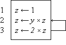
Program 1.3 illustrates the use of a branch point. Statement α5 is a comparison which determines the branch to statements β1, δ1, or γ1, according as z > n, z = n, or z < n. The program represents a crude by effective process for determining x = n2/3 for any positive cube n.
Program 1.3 Program for x = n2/3
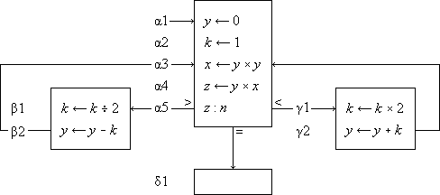
Program 1.4 shows the preceding program reorganized into a compact linear array and introduces two further conventions on the labeling of branch points. The listed successor of a branch statement is selected if none of the labeled conditions is met. Thus statement 6 follows statement 5 if neither of the arrows (to exit or to statement 8) are followed, i.e. if z < n. Moreover, any unlabeled arrow is always followed; e.g., statement 7 is invariably followed by statement 3, never by statement 8.
A program begins at a point indicated by an entry arrow (step 1) and ends at a point indicated by an exit arrow (step 5). There are two useful consequences of confining a program to the form of a linear array: the statements may be referred to by a unique serial index (statement number), and unnecessarily complex organization of the program manifests itself in crossing branch lines. The importance of the latter characteristic in developing clear and comprehensible programs is not sufficiently appreciated.
 | |
| Program 1.4 Linear arrangement of Program 1.3 |
 | |
| Program 1.5 Matrix multiplication |
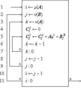
A process which is repeated a number of times is said to be iterated, and a process (such as in Program 1.4) which includes one or more iterated subprocesses is said to be iterative. Program 1.5 shows an iterative process for the matrix multiplication
C ← AB
defined in the usual way as
Cji =  Aki ×
Bjk ,
Aki ×
Bjk ,
|
i = 1,2, …, μ(A), j = 1,2, …, ν(B), |
where the dimensions of an
|
Program 1.5. Steps 1-3 initialize the indices, and the loop 5-7 continues to add successive products to the partial sum until k reaches zero. When this occurs, the process continues through step 8 to decrement j and to repeat the entire summation for the new value of j, providing that it is not zero. If j is zero, the branch to step 10 decrements i and the entire process over j and k is repeated from j = ν(B), providing that i is not zero. If i is zero, the process is complete, as indicated by the exit arrow. |
In all examples used in this chapter, emphasis will be placed on clarity of description of the process, and considerations of efficient execution by a computer or class of computers will be subordinated. These considerations can often be introduced later by relatively routine modifications of the program. For example, since the execution of a computer operation involving an indexed variable is normally more costly than the corresponding operation upon a nonindexed variable, the substitution of a variable s for the variable Cji specified by statement 5 of Program 1.5 would accelerate the execution of the loop. The variable s would be initialized to zero before each entry to the loop and would be used to specify Cji at each termination.
The practice of first setting an index to its maximum value and then decrementing it (e.g., the index k in Program 1.5) permits the termination comparison to be made with zero. Since zero often occurs in comparisons, it is convenient to omit it. Thus, if a variable stands alone at a branch point, comparison with zero is implied. Moreover, since a comparison on an index frequently occurs immediately after it is modified, a branch at the point of modification will denote branching upon comparison of the indicated index with zero, the comparison occurring after modification. Designing programs to execute decisions immediately after modification of the controlling variable results in efficient execution as well as notational elegance, since the variable must be present in a central register for both operations.
Since the sequence of execution of statements is indicated by connecting arrows as well as by the order of listing, the latter can be chosen arbitrarily. This is illustrated by the functionally identical Programs 1.3 and 1.4. Certain principles of ordering may yield advantages such as clarity or simplicity of the pattern of connections. Even though the advantages of a particular organizing principle are not particularly marked, the uniformity resulting from its consistent application will itself be a boon. The scheme here adopted is called the method of leading decisions: the decision on each parameter is placed as early in the program as practicable, normally just before the operations indexed by the parameter. This arrangement groups at the head of each iterative segment the initialization, modification, and the termination test of the controlling parameter. Moreover, it tends to avoid program flaws occasioned by unusual values of the argument.
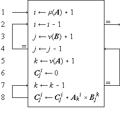 | |
| Program 1.6 Matrix multiplication using leading decisions |
For example, Program 1.6 (which is a reorganization of Program 1.5) behaves properly for matrices of dimension zero, whereas Program 1.5 treats every matrix as if it were of dimension one or greater.
Although the labeled arrow representation of program branches provides a complete and graphic description, it is deficient in the following respects: (1) a routine translation to another language (such as computer code) would require the tracing of arrows, and (2) it does not permit programmed modification of the branches.
The following alternative form of a branch statement will therefore be used as well:
x : y, r → s.
This denotes a branch to statement number si of the program if the relation xr i y holds. The parameters r and s may themselves be defined and redefined in other parts of the program. The null element ∘ will be used to denote the relation which complements the remaining relations r i; in particular, (∘)→(s), or simply →s, will denote an unconditional branch to statement s. Program 1.7 shows the use of these conventions in a reformulation of Program 1.6. More generally, two or more otherwise independent programs may interact through a statement in one program specifying a branch in a second. The statement number occurring in the branch must then be augmented by the name of the program in which the branch is effected. Thus the statement (∘) → Program 2.24 executed in Program 1 causes a branch to step 24 to occur in Program 2.
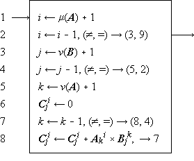 | |
| Program 1.7 A reformulation of Program 1.6, using an algebraic statement of the branching |
One statement in a program can be modified by another statement which changes certain of its parameters, usually indices. More general changes in statements can be effected by considering the program itself as a vector p whose components are the individual, serially numbered statements. All the operations to be defined on general vectors can then be applied to the statements themselves. For example, the jth statement can be respecified by the ith through the occurrence of the statement pj ← pi.
The interchange of two quantities y and x
(that is, x specifies y and
the original value of y specifies x)
will be denoted by the statement y ↔ x.
1.3 Structure of the language
Conventions
The Summary of Notation at the end of the book summarizes the notation developed in this chapter. Although intended primarily for reference, it supplements the text in several ways. It frequently provides a more concise alternative definition of an operation discussed in the text, and it also contains important but easily grasped extensions not treated explicitly in the text. By grouping the operations into related classes it displays their family relationships.
A concise programming language must incorporate families of operations whose members are related in a systematic manner. Each family will be denoted by a specific operation symbol, and the particular member of the family will be designated by an associated controlling parameter (scalar, vector, matrix, or tree) which immediately precedes the main operation symbol. The operand is placed immediately after the main operation symbol. For example, the operation k ↑ x (left rotation of x by k places) may be viewed as the kth member of the set of rotation operators denoted by the symbol ↑.
Operations involving a single operand
and no controlling parameter
(such as
In interpreting a compound operation such as k ↑ (j ↓ x) it is important to recognize that the operation symbol and its associated controlling parameter together represent an indivisible operation and must not be separated. It would, for example, be incorrect to assume that j ↑ (k ↓ x) were equivalent to k ↑ (j ↓ x), although it can be shown that the complete operations j ↓ and k ↑ do commute, that is k ↑ (j ↓ x) = j ↓ (k ↑ x).
The need for parentheses will be reduced by assuming that compound statements are, except for intervening parentheses, executed from right to left. Thus k ↑ j ↓ x is equivalent to k ↑ (j ↓ x), not to (k ↑ j) ↓ x.
Structured operands such as vectors and matrices, together with a systematic component-by-component generalization of elementary operations, provide an important subordination of detail in the description of algorithms. The use of structured operands will be facilitated by selection operations for extracting a specified portion of an operand, reduction operations for extending an operation (such as logical or arithmetic multiplication) over all components, and permutation operations for reordering components. Operations defined on vectors are extended to matrices: the extended operation is called a row operation if the underlying vector operation is applied to each row of the matrix and a column operation if it is applied to each column. A column operation is denoted by doubling the symbol employed for the corresponding row (and vector) operation.
A distinct typeface will be used for each class of operand as detailed in Table 1.8. Special quantities (such as the prefix vectors ⍺i defined in Sec. 1.7) will be denoted by Greek letters in the appropriate typeface. For mnemonic reasons, an operation closely related to such a special quantity will be denoted by the same Greek letter. For example, ⍺/u denotes the maximum prefix (Sec. 1.10) of the logical vector u. Where a Greek letter is indistinguishable from a Roman, sanserif characters will be used, e.g. E and I for the capitals of epsilon and iota.
| Type of Operand | Representation | ||||||||||||||||||||||||||||||||||||||||||||||
| Printed | Typed | ||||||||||||||||||||||||||||||||||||||||||||||
|
|
|
|||||||||||||||||||||||||||||||||||||||||||||
Table 1.8 Typographic conventions for classes of operands
Literals and variables
The power of any mathematical notation rests largely on the use of symbols to represent general quantities which, in given instances, are further specified by other quantities. Thus Program 1.4 represents a general process which determines x = n2/3 for any suitable value of n. In a specific case, say n = 27, the quantity x is specified as the number 9.
Each operand occurring in a meaningful process must be specified ultimately in terms of commonly accepted concepts. The symbols representing such accepted concepts will be called literals. Examples of literals are the integers, the characters of the various alphabets, punctuation marks, and miscellaneous symbols such as $ and %. The literals occurring in Program 1.4 are 0, 1, 2.
It is important to distinguish clearly between general symbols and literals. In ordinary algebra this presents little difficulty, since the only literals occurring are the integers and the decimal point, and each general symbol employed includes an alphabetic character. In describing more general processes, however, alphabetic literals (such as proper names) also appear. Moreover, in a computer program, numeric symbols (register addresses) are used to represent the variables.
In general, then, alphabetic literals, alphabetic variables, numeric literals, and numeric variables may all appear in a complex process and must be clearly differentiated. The symbols used for literals will be Roman letters (enclosed in quotes when appearing in text) and standard numerals. The symbols used for variables will be italic letters, italic numerals, and boldface letters as detailed in Table 1.8. Miscellaneous signs and symbols when used as literals will be enclosed in quotes in both programs and text.
It is sometimes desirable
(e.g., for mnemonic reasons) to denote
a variable by a string of alphabetic
or other symbols rather than by a single symbol.
The monolithic interpretation of such a string
will be indicated by the tie
used in musical notation, thus:
 and
and
 may denote the variable “inventory”,
a vector of inventory values,
and a matrix of inventory values,
respectively.
may denote the variable “inventory”,
a vector of inventory values,
and a matrix of inventory values,
respectively.
In the set of alphabetic characters, the space plays a special role. For other sets a similar role is usually played by some one element, and this element is given the special name of null element. In the set of numeric digits, the zero plays a dual role as both null element and numeric quantity. The null element will be denoted by the degree symbol ∘.
In any determinate process, each operand must be specified ultimately in terms of literals. In Program 1.4, for example, the quantity k is specified in terms of known arithmetic operations (multiplication and division) involving the literals 1 and 2. The quantity n, on the other hand, is not determined within the process and must presumably be specified within some larger process which includes Program 1.4. Such a quantity is called an argument of the process.
Domain and range
The class of arguments and the class of results of a given operator are called its domain and range, respectively. Thus the domain and range of the magnitude operation (|x|) are the real numbers and the nonnegative real numbers, respectively.
A variable is classified according
to the range of values it may assume:
it is logical, integral, or numerical,
according as the range is the set of logical variables
(that is, 0 and 1), the set of integers,
or the set of real numbers.
Each of the foregoing classes is clearly
a subclass of each class following it,
and any operation defined on a class clearly
applies to any of its subclasses.
A variable which is nonnumeric
will be called arbitrary.
In the Summary of Notation,
the range and domain of each of the operators
defined is specified in terms of the foregoing classes
according to the conventions shown in Sec. S.1.
1.4 Elementary operations
The elementary operations employed include the ordinary arithmetic operations, the elementary operations of the logical calculus, and the residue and related operations arising in elementary number theory. In defining operations in the text, the symbol ↔ will be used to denote equivalence of the pair of statements between which it occurs.
Arithmetic operations
The ordinary arithmetic operations will be denoted by the ordinary symbols +, –, ×, and ÷ and defined as usual except that the domain and range of multiplication will be extended slightly as follows. If one of the factors is a logical variable (0 or 1), the second may be arbitrary and the product then assumes the value of the second factor or zero according as the value of the first factor (the logical variable) is 1 or 0. Thus if the arbitrary factor is the literal “q”, then| 0 × q = q × 0 = 0 | |
| and | 1 × q = q × 1 = q |
According to the usual custom in ordinary algebra, the multiplication symbol may be elided.
Logical operations
The elementary logical operations and, or, and not will be denoted by ∧, ∨ and an overbar and are defined in the usual way as follows:
| w ← u ∧ v | ↔ | w = 1 if and only if u = 1 and | v = 1, |
| w ← u ∨ v | ↔ | w = 1 if and only if u = 1 or | v = 1, |
w ←  | ↔ | w = 1 if and only if u = 0. |
If x and y are numerical quantities,
then the expression x < y implies
that the quantity x stands in the relation
“less than” to the quantity y.
More generally, if α and β are arbitrary entities
and R is any relation defined on them,
the relational statement
(x > 0) – (x < 0)
(commonly called the sign function or sgn x) assumes the values 1, 0, or –1 according as x is strictly positive, 0, or strictly negative. Moreover, the magnitude function |x| may be defined as |x| = x × sgn x = x × ((x > 0) – (x < 0)).
The relational statement is a useful generalization
of the Kronecker delta, that is
Residues and congruence
For each set of integers n, j, and b, with b > 0, there exists a unique pair of integers q and r such that
n = bq + r, j ≤ r < j + b.
The quantity r is called the j-residue of n modulo b and is denoted by b | j n. For example, 3 |0 9 = 0, 3 |1 9 = 3, and 3 |0 10 = 1. Moreover, if n ≥ 0, then b |0 n is the remainder obtained in dividing n by b and q is the integral part of the quotient. A number n is said to be of even parity if its 0-residue modulo 2 is zero and of odd parity if 2 |0 n = 1.
If two numbers n and m have the same j-residue modulo b, they differ by an integral multiple of b and therefore have the same k-residue module b for any k. If b | j n = b | j m, then m and n are said to be congruent mod b. Congruency is transitive and reflexive and is denoted by
m ≡ n (mod b).
In classical treatments, such as Wright (1939), only the 0-residue is considered. The use of 1-origin indexing (cf. Sec. 1.5) accounts for the interest of the 1-residue.
A number represented in a positional notation (e.g., in a base ten or a base two number system) must, in practice, employ only a finite number of digits. It is therefore often desirable to approximate a number x by an integer. For this purpose two functions are defined:
| 1. | the floor of x (or integral part of x), denoted by ⌊x⌋ and defined as the largest integer not exceeding x, | |
| 2. | the ceiling of x, denoted by ⌈x⌉ and defined as the smallest integer not exceeded by x. |
Thus
| ⌈3.14⌉ = 4, | ⌊3.14⌋ = 3, | ⌊–3.14⌋ = –4, | |||
| ⌈3.00⌉ = 3, | ⌊3.00⌋ = 3, | ⌊–3.00⌋ = –3. |
Clearly ⌈x⌉ =
–⌊–x⌋ and
⌊x⌋
≤ x ≤ ⌈x⌉.
Moreover, n = b⌊n ÷ b⌋
+ b |0 n for all integers n.
Hence the integral quotient
⌊n ÷ b⌋
is equivalent to the quantity q occurring in the definition
of the j-residue for the case j = 0.
1.5 Structured operands
Elementary operations
Any operation defined on a single operand can be generalized to apply to each member of an array of related operands. Similarly, any binary operation (defined on two operands) can be generalized to apply to pairs of corresponding elements of two arrays. Since algorithms commonly incorporate processes which are repeated on each member of an array of operands, such generalization permits effective subordination of detail in their description. For example, the accounting process defined on the data of an individual bank account treats a number of distinct operands within the account, such as account number, name, and balance. Moreover, the over-all process is defined on a large number of similar accounts, all represented in a common format. Such structured arrays of variables will be called structured operands, and extensive use will be made of three types, called vector, matrix, and tree. As indicated in Sec. S.1 of the Summary of Notation, a structured operand is further classified as logical, integral, numerical, or arbitrary, according to the type of elements in contains.
A vector x is the ordered array of elements (x1, x2, x3, …, xν(x)). The variable xi is called the ith component of the vector x, and the number of components, denoted by ν(x) (or simply by ν when the determining vector is clear from context), is called the dimension of x. Vectors and their components will be represented in lower case boldface italics. A numerical vector x may be multiplied by a numerical quantity k to produce the scalar multiple k × x (or kx) defined as the vector z such that z i = k × xi.
All elementary operations defined on individual variables are extended consistently to vectors as component-by-component operations. For example,
| z = x + y | ↔ | zi = xi + yi, | |
| z = x × y | ↔ | zi = xi × yi, | |
| z = x ÷ y | ↔ | zi = xi ÷ yi, | |
| z = ⌈x⌉ | ↔ | zi = ⌈xi⌉ | |
| w = u ∧ v | ↔ | wi = ui ∧ vi, | |
| w = (x < y) | ↔ | wi = (xi < yi). |
Thus if x = (1, 0, 1, 1) and y = (0, 1, 1, 0) then x + y = (1, 1, 2, 1), x ∧ y = (0, 0, 1, 0), and (x < y) = (0, 1, 0, 0).
Matrices
A matrix M is the ordered two-dimensional array of variables
|


The vector
The variable M ji
is called the (i,j)th component
or element of the matrix.
A matrix and its elements will be represented
by upper case boldface italics.
Operations defined on each element of a matrix
are generalized component by component
to the entire matrix.
Thus, if  is any binary operator,
P = M
N ↔
Mji
Nji.
Index systems
The subscript appended to a vector to designate a single component is called an index, and the indices are normally chosen as a set of successive integers beginning at 1, that is, x = (x1, x2, … xν). It is, however, convenient to admit more general j-origin indexing in which the set of successive integers employed as indices in any structured operand begin with a specified integer j.
The two systems of greatest interest
are the common 1-origin system,
which will be employed
almost exclusively in this chapter,
and the 0-origin system.
The latter system is particularly convenient
whenever the index itself must be represented
in a positional number system and will therefore
be employed exclusively in the treatment
of computer organization in Chapter 2.
1.6 Rotation
The left rotation of a vector x
is denoted by k ↑ x
and specifies the vector obtained by cyclical
left shift of the components of x
by k places.
Thus if
z = k ↑ x ↔ z i = x j, where j = ν|1(i + k).
Right rotation is denoted by k ↓ x and is defined analogously. Thus
z = k ↓ x ↔ z i = x j, where j = ν|1(i – k).
If k = 1, it may be elided. Thus ↑ b = (a, n, d, y, c).
Left rotation is extended to matrices in two ways as follows:
| A ← j ↑ B | ↔ | Ai = ji ↑ Bi | |
C ← k  B B |
↔ | Ci = kj ↑ Bj |
The first operation is an extension
of the basic vector rotation to each row
of the matrix and is therefore called row rotation.
The second operation is the corresponding
column operation and is therefore denoted
by the doubled operation symbol .
For example, if
k = (0, 1, 2),
and| B = |
|
| and |
| . |
Right rotation is extended analogously.
1.7 Special vectors
Certain special vectors warrant special symbols.
In each of the following definitions,
the parameter n will be used to specify the dimension.
The interval vector
⍳j(n)
is defined as the vector of integers
beginning with j.
Thus ⍳0(4)=(0, 1, 2, 3),
⍳1(4)=(1, 2, 3, 4),
and ⍳–7(5)=
(–7, –6, –5, –4, –3).
Four types of logical vectors are defined as follows.
The jth unit vector
∊ j(n)
has a one in the jth position, that is,
(∊ j(n))k
= (k = j).
The full vector ∊(n)
consists of all ones.
The vector consisting of all zeros is denoted
both by 0 and by  (n).
The prefix vector of weight j is denoted by
⍺ j(n)
and possesses ones in the first k positions,
where k is the lesser
of j and n.
The suffix vector
⍵ j(n)
is defined analogously.
Thus ∊2(3) = (0, 1, 0),
∊(4) = (1, 1, 1, 1),
⍺3(5) = (1, 1, 1, 0, 0),
⍵3(5) = (0, 0, 1, 1, 1), and
⍺7(5) =
⍺5(5) = (1, 1, 1, 1, 1).
Moreover,
⍵ j(n) =
j ↑ ⍺ j(n),
and ⍺ j(n) =
j ↓ ⍵ j(n).
(n).
The prefix vector of weight j is denoted by
⍺ j(n)
and possesses ones in the first k positions,
where k is the lesser
of j and n.
The suffix vector
⍵ j(n)
is defined analogously.
Thus ∊2(3) = (0, 1, 0),
∊(4) = (1, 1, 1, 1),
⍺3(5) = (1, 1, 1, 0, 0),
⍵3(5) = (0, 0, 1, 1, 1), and
⍺7(5) =
⍺5(5) = (1, 1, 1, 1, 1).
Moreover,
⍵ j(n) =
j ↑ ⍺ j(n),
and ⍺ j(n) =
j ↓ ⍵ j(n).
A logical vector of the form ⍺h(n) ∧ ⍵ j(n) is called an infix vector. An infix vector can also be specified in the form j ↓ ⍺k(n), which displays its weight and location more directly.
An operation such as x ∧ y is defined only for compatible vectors x and y, that is, for vectors of like dimension. Since this compatibility requirement can be assumed to specify implicitly the dimension of one of the operands, elision of the parameter n may be permitted in the notation for the special vectors. Thus, if y = (3, 4, 5, 6, 7), the expression ∊ × y and ∊ j × y imply that the dimensions of ∊ and ∊ j are both 5. Moreover, elision of j will be permitted for the interval vector ⍳ j(n) (or ⍳ j), and for the residue operator | j when j is the index origin in use.
It is, of course, necessary to specify the index origin in use at any given time. For example, the unit vector ∊3(5) is (0, 0, 1, 0, 0) in a 1-origin system and (0, 0, 0, 1, 0) in a 0-origin system, even though the definition (that is, (∊ j(n))k = (k = j)) remains unchanged. The prefix and suffix vectors are, of course, independent of the index origin. Unless otherwise specified, 1-origin indexing will be assumed.
The vector ∊(0) is a vector
of dimension zero and will be called
the null vector.
It should not be confused
with the special null element ∘.
1.8 Reduction
An operation (such as summation) which is applied
to all components of a vector to produce a result
of a simpler structure is called a reduction.
The -reduction
of a vector x is denoted by
/x
and defined as
z ←
/x
↔ z =
(… ((x1
x2)
x3)
…)
xν),
where
is any binary operator with a suitable domain.
Thus +/x is the sum,
×/x is the product,
and ∨/x
is the logical sum of the components
of a vector x.
For example, ×/⍳1(5)
= 1 × 2 × 3 × 4 × 5,
×/⍳1(n) = n!,
and +/⍳1(n) =
n(n + 1)/2.
As a further example, De Morgan’s law
may be expressed as ∧/u
= ![]() ,
where u is
a logical vector of dimension two.
Moreover, a simple inductive argument (Exercise 1.10)
shows that the foregoing expression is the
valid generalization of De Morgan’s law
for a logical vector u
of arbitrary dimension.
,
where u is
a logical vector of dimension two.
Moreover, a simple inductive argument (Exercise 1.10)
shows that the foregoing expression is the
valid generalization of De Morgan’s law
for a logical vector u
of arbitrary dimension.
A relation R incorporated
into a relational statement (xRy)
becomes, in effect, an operator on the variables
x and y.
Consequently, the reduction R/x
can be defined in a manner analogous to that of
(/x),
that is,
R/x = (… ((x1 R x2) R x3) R …) R xν).
The parentheses now imply relational statements as well as grouping. The relational reductions of practical interest are ≠/u, and =/u, the exclusive-or and the equivalence reduction, respectively.
The inductive argument of Exercise 1.10 shows that ≠/u = 2 |0 (+/u). For example, if u = (1,0,1,1,0), then
| ≠/u | = | ((((1 ≠ 0) ≠ 1) ≠ 1) ≠ 0) | |
| = | (((1 ≠ 1) ≠ 1) ≠ 0) | ||
| = | ((0 ≠ 1) ≠ 0) | ||
| = | (1 ≠ 0) = 1, | ||
and 2 |0 (+/u) = 2 |0 3 = 1.
Similarly, =/u = ![]() ,
and as a consequence,
,
and as a consequence,
≠/u = ![]() ,
,
a useful companion to De Morgan’s law.
To complete the system it is essential to define
the value of
/∊(0),
the reduction of the null vector of dimension zero,
as the identity element of the operator
or relation .
Thus +/∊(0) = ∨/∊(0) = 0,
and ×/∊(0) =
∧/∊(0) = 1.
A reduction operation is extended
to matrices in two ways.
A row reduction of a matrix X
by an operator
is denoted by
y ←
/X
and specifies a vector y of dimension
μ(X) such that
yi =
/Xi.
A column reduction of X is denoted
by z ←
//X
and specifies a vector z
of dimension ν(X)
such that z j =
//X j.
For example, if
| U = |  |
1 0 1 0 |  |
| 0 0 1 1 | |||
| 1 1 1 0 |
then +/U =
1.9 Selection
Compression
The effective use of structured operands depends not only on generalized operations but also on the ability to specify and select certain elements or groups of elements. The selection of single elements can be indicated by indices, as in the expressions vi, M i, M j, and M i j. Since selection is a binary operation (i.e., to select or not to select), more general selection is conveniently specified by a logical vector, each unit component indicating selection of the corresponding component of the operand.
The selection operation defined on an arbitrary
vector a and a compatible
(i.e., equal in dimension)
logical vector u is denoted by
c ← u/a
and is defined as follows:
the vector c is obtained from
a by suppressing from
a each component
ai
for which ui = 0.
The vector u is said to compress
the vector a.
Clearly ν(c) = +/u.
For example, if u =
Row compression of a matrix,
denoted by u/A,
compresses each row vector Ai
to form a matrix of dimension
|
|
| u/v//A = v//u/A = |  |
|
 |
. |
It is clear that row compression suppresses columns corresponding to zeros of the logical vector and that column compression suppresses rows. This illustrates the type of confusion in nomenclature which is avoided by the convention adopted in Sec. 1.3: an operation is called a row operation if the underlying operation from which it is generalized is applied to the row vectors of the matrix, and a column operation if it is applied to columns.
|
Example 1.1. A bank makes a quarterly review of accounts to produce the following four lists:
The ledger may be described by a matrix
with column vectors L1, L2, and L3, representing names, account numbers, and balances, respectively, and with row vectors L1, L2, …, Lm, representing individual accounts. An unassigned account number is identified by the word “none” in the name position. The four output lists will be denoted by the matrices P, Q, R, and S, respectively. They can be produced by Program 1.9. |


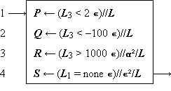 |
Legend |
Program 1.9 Selection on bank ledger L (Example 1.1)
|
Program 1.9. Since L3 is the vector of balances, and 2∊ is a compatible vector each of whose components equals two, the relational statement (L3 < 2∊) defines a logical vector having unit components corresponding to those accounts to be included in the list P. Consequently, the column compression of step 1 selects the appropriate rows of L to define P. Step 2 is similar, but step 3 incorporates an additional row compression by the compatible prefix vector ⍺² = (1,1,0) to select columns one and two of L. Step 4 represents the comparison of the name (in column L1) with the literal “none”, the selection of each row which shows agreement, and the suppression of all columns but the second. The expression “none ∊” occurring in step 4 illustrates the use of the extended definition of multiplication. |
Mesh, mask, and expansion
A logical vector u
and the two vectors
a =
 /c and
b = u/c,
obtained by compressing a vector c,
collectively determine the vector c.
The operation which specifies c
as a function of a, b, and
u is called a mesh
and is defined as follows:
If a and b are
arbitrary vectors and if u
is a logical vector such that +/
= ν(a) and +/u
= ν(b), then the mesh of
a and b on
u is denoted by
/c
= a and u/c
= b.
The mesh operation is equivalent to choosing successive
components of c from a
or b according as the successive components
of u are 0 or 1.
If, for example, a =
/c and
b = u/c,
obtained by compressing a vector c,
collectively determine the vector c.
The operation which specifies c
as a function of a, b, and
u is called a mesh
and is defined as follows:
If a and b are
arbitrary vectors and if u
is a logical vector such that +/
= ν(a) and +/u
= ν(b), then the mesh of
a and b on
u is denoted by
/c
= a and u/c
= b.
The mesh operation is equivalent to choosing successive
components of c from a
or b according as the successive components
of u are 0 or 1.
If, for example, a =
(a) |
(b) | ||||||||||||||||||
Legend |
Program 1.10 Interfiling program
Program 1.10a (which describes the merging of
the vectors a and b,
with the first and every third component thereafter
chosen from a) can be described
alternatively as shown in Program 1.10b.
Since ⍳1 =
Mesh operations on matrices are defined analogously, row mesh and column mesh being denoted by single and double reverse virgules, respectively.
The catenation of vectors
 y …
z
y …
z
x
y …
z =
(x1, x2, …,
xν(x),
y1, y2, …,
zν(z)).
Catenation is clearly associative and for two vectors x and y it is a special case of the mesh \x, u, y\ in which u is a suffix vector.
In numerical vectors (for which addition of two vectors is defined), the effect of the general mesh operation can be produced as the sum of two meshes, each involving one zero vector. Specifically,
| \x, u, y\ | = | \x, u, 0\ + \0, u, y\ |
| = | \0, , x\ +
\0, u, y\. |
The operation \0, u, y\
proves very useful in numerical work and will be called
expansion of the vector y,
denoted by u\y.
Compression of u\y
by u and by
clearly yields y and 0, respectively.
Moreover, any numerical vector x
can be decomposed by a compatible vector
u according to the relation
x =
\/x +
u\u/x.
The two terms are vectors of the same dimension which have no nonzero components in common. Thus if u = (1, 0, 1, 0, 1), the decomposition of x appears as
x = (0, x2, 0, x4, 0) + (x1, 0, x3, 0, x5).
Row expansion and column expansion of matrices are defined and denoted analogously. The decomposition relations become
X =
\/X +
u\u/X,
and
X =
\\//X +
u\\u//X.
The mask operation is defined formally as follows:
c ←
/a, u, b/ ↔
/c =
/a, and
u/c = u/b.
The vectors c, a, u, and b are clearly of a common dimension and ci = ai or bi according as ui = 0 or ui = 1. Moreover, the compress, expand, mask, and mesh operations on vectors are related as follows:
| /a, u, b/ | = | \/a,
u, u/b\, |
| \a, u, b\ | = | /\a,
u, u\b/. |
Analogous relations hold for the row mask and row mesh and for the column mask and column mesh.
Certain selection operations are controlled by logical matrices rather than by logical vectors. The row compression U/A selects elements of A corresponding to the nonzero elements of U. Since the nonzero elements of U may occur in an arbitrary pattern, the result must be construed as a vector rather than a matrix. More precisely, U/A denotes the catenation of the vectors U i/Ai obtained by row-by-row compression of A by U. The column compression U//A denotes the catenation of the vectors Uj/Aj. If, for example
| U = | |
0 1 0 1 1 | |
| 1 1 0 0 0 | |||
| 0 1 1 0 0 |
then
U/A =
(A21,
A41,
A51,
A12,
A22,
A23,
A33),
and
U//A =
(A12,
A21,
A22,
A23,
A33,
A41,
A51).
Compression by the full matrix E
(defined by  = 0)
produces either a row list
(E/A)
or a column list
(E//A)
of the matrix A.
Moreover, a numerical matrix X
can be represented jointly by the logical matrix
U and the row list
U/X
(or the column list U//X),
where U = (X ≠ 0).
If the matrix X is sparse
(i.e., the components are predominantly zero),
this provides a compact representation
which may reduce the computer storage
required for X.
= 0)
produces either a row list
(E/A)
or a column list
(E//A)
of the matrix A.
Moreover, a numerical matrix X
can be represented jointly by the logical matrix
U and the row list
U/X
(or the column list U//X),
where U = (X ≠ 0).
If the matrix X is sparse
(i.e., the components are predominantly zero),
this provides a compact representation
which may reduce the computer storage
required for X.
The compression operations controlled
by matrices also generate a group of
corresponding mesh and mask operations
as shown in Sec. S.9.
1.10 Selection vectors
The logical vector u involved in selection operations may itself arise in various ways. It may be a prefix vector ⍺ j, a suffix ⍵ j, or an infix (i ↓ ⍺ j); the corresponding compressed vectors ⍺ j/x, ⍵ j/x, and (i ↓ ⍺ j)/x are called a prefix, suffix, and infix of x, respectively.
Certain selection vectors arise as functions of other vectors, e.g., the vector (x ≥ 0) can be used to select all nonnegative components of x, and (b ≠ *∊) serves to select all components of b which are not equal to the literal “*”. Two further types are important: the selection of the longest unbroken prefix (or suffix) of a given logical vector, and the selection of the set of distinct components occurring in a vector. The first is useful in left (or right) justification or in a corresponding compression intended to eliminate leading or trailing “filler components” of a vector (such as left zeros in a number or right spaces in a short name).
For any logical vector u, the maximum prefix of u is denoted by ⍺/u and defined as follows:
u ← ⍺/u ↔ v = ⍺ j
where j is the maximum value for which ∧/(⍺ j/u) = 1. The maximum suffix is denoted by ⍵/u and is defined analogously. If, for example, u = (1, 1, 1, 0, 1, 1, 0, 0, 1, 1), then ⍺/u = (1, 1, 1, 0, 0, 0, 0, 0, 0, 0), ⍵/u = (0, 0, 0, 0, 0, 0, 0, 0, 1, 1), +/⍺/u = 3, and +/⍵/u = 2.
The leading zeros of a numerical vector x can clearly be removed either by compression:
![]()
or by left justification (normalization):
z ← (+/⍺/(x = 0)) ↑ x.
The extension of the maximum prefix operation
to the rows of a logical matrix U
is denoted by ⍺/U
and defined as the compatible logical matrix
V, such that
V i
= ⍺/U i.
The corresponding maximum column prefix operation
is denoted by ⍺//U.
Right justification of a numerical matrix
X is achieved by the rotation
k ↓ X,
where k = +/⍵/(X = 0),
and top justification is achieved
by the rotation
((+//⍺//(X = 0)
X
(see Sec. S.6.)
A vector whose components are all distinct will be called an ordered set. The forward set selector on b is a logical vector denoted by σ/b and defined as follows: the statement v ← σ/b implies that vj = 1 if and only if bj differs from all preceding components of b. Hence v/b is a set which contains all distinct components of b, and +/v/⍳ is a minimum. For example, if c = (C, a, n, a, d, a), then (σ/c)/c = (C, a, n, d) is a list of the distinct letters in c in order of occurrence. Clearly (σ/b)/b = b if and only if b is a set.
The backward set selector τ/b
is defined analogously
(e.g., (τ/c)/c =
1.11 The generalized matrix product
The ordinary matrix product of matrices X and Y is commonly denoted by XY and defined as follows:
|
Z ← XY ↔
Z j i =
|
i = 1, 2, …, μ(X) j = 1, 2, …, ν(Y). |
(XY)j i = +/(X i × Yj).
This formulation emphasizes the fact that
matrix multiplication incorporates two elementary operations
(+, ×) and suggests that they be displayed explicitly.
The ordinary matrix product will therefore be written as
X  Y.
Y.
More generally, if 1
and 2
are any two operators
(whose domains include the relevant operands),
then the generalized matrix product
 is defined as follows:
( |
i = 1, 2, …, μ(X) j = 1, 2, …, ν(Y). |
| and |
|
|
|
 B =
B =
|
|
 B =
B =  B =
B = The generalized matrix product and the selection operations together provide an elegant formulation in several established areas of mathematics. A few examples will be chosen from two such areas, symbolic logic and matrix algebra.
In symbolic logic, De Morgan’s laws
(∧/u = ![]() and
=/u =
and
=/u =  )
can be applied directly to show that
)
can be applied directly to show that
U  V
=
V
= ![]() .
.
In matrix algebra, the notion of partitioning a matrix into submatrices of contiguous rows and columns can be generalized to an arbitrary partitioning specified by a logical vector u. The following easily verifiable identities are typical of the useful relations which result:
| X Y |
= | (/X)
(//Y) +
(u/X)
(u//Y),
| |||
| u/(X Y) |
= | X (u/Y), |
|||
| u//(X Y) |
= | (u//X) Y. |
The first identity depends on the commutativity and associativity of the operator + and can clearly be generalized to other associative commutative operators, such as ∧, ∨, and ≠.
The generalized matrix product applies directly
(as does the ordinary matrix product
X Y)
to vectors considered as row (that is, 1 × n)
or as column matrices. Thus:
z ← X  y y |
↔ | z i | = |
1/(X i
2 y), |
|
| z ← y X |
↔ | z j | = |
1/(y
2 Xj ), |
|
| z ← y x |
↔ | z | = |
1/(y
2 x). |
The question of whether a vector enters a given operation
as a row vector or as a column vector is normally settled
by the requirement of conformability,
and no special indication is required.
Thus y enters as a column vector
in the first of the preceding group of definitions
and as a row vector in the last two.
The question remains, however, in the case
of the two vector operands, which may be considered
with the pre-operand either as a row
(as in the scalar product
y x)
or as a column.
The latter case produces a matrix Z
and will be denoted by
Z ←
y  2 x,
2 x,
where Zji =
yi
2
xj,
μ(Z) = ν(y), and
ν(Z) = ν(x).[b]
For example, if each of the vectors indicated
is of dimension three, then
|
| ||||||||||||||||
| |||||||||||||||||
1.12 Transpositions
Since the generalized matrix product is defined on columns of the post-operand and rows of the pre-operand, convenient description of corresponding operations on the rows of the post-operand and columns of the pre-operand demands the ability to transpose a matrix B, that is, to specify a matrix C such that Ci j = Bji. In ordinary matrix algebra this type of transposition suffices, but in more general work transpositions about either diagonal and about the horizontal and the vertical are also useful. Each of these transpositions of a matrix B is denoted by a superior arrow whose inclination indicates the axis of the transposition. Thus:
C ←  |
Ci j = Bj i | i = 1, 2, …, μ(B) j = 1, 2, …, ν(B) |
|||
C ←  | |||||
C ←  | |||||
C ←  |
For a vector x, either  or
or  will denote reversal of the order
of the components.
For ordinary matrix transposition (that is, ),
the commonly used notation
will denote reversal of the order
of the components.
For ordinary matrix transposition (that is, ),
the commonly used notation  will also be employed.
Since transpositions can effect any one or more
of three independent alternatives
(i.e., interchange of row and column indices
or reversal of order of row or of column indices),
repeated transpositions can produce
eight distinct configurations.
There are therefore seven distinct
transformations possible;
all can be generated by any pair
of transpositions having nonperpendicular
axes.[c]
1.13 Special logical matrices
Certain of the special logical vectors introduced in Sec. 1.7 have useful analogs in logical matrices. Dimensions will again be indicated in parentheses (with the column dimension first) and may be elided whenever the dimension is determined by context. If not otherwise specified, a matrix is assumed to be square.
Cases of obvious interest are the full matrix
E(m × n),
defined by (m × n) = 0,
and the identity matrix
I(m × n),
defined by Iji
= (i = j).
More generally, superdiagonal matrices
kI(m × n)
are defined such that
kIji(m × n)
= (j = i + k), for k ≥ 0.
Clearly 0I =
I.
Moreover, for square matrices,
hI
kI =
(h + k)I.
Four triangular matrices will be defined, the geometrical symbols employed for each indicating the (right-angled isosceles) triangular area of the m × n rectangular matrix which is occupied by ones. Thus
C ←  (m × n) (m × n) |
↔ | C j i | = (i + j ≤ min(m, n)) | for i = 1, 2, …, m and j = 1, 2, …, n. |
||
C ←  (m × n) (m × n) |
↔ | |||||
C ←  (m × n) (m × n) |
↔ | |||||
C ←  (m × n) (m × n) |
↔ |
The use of the matrices E and
I
will be illustrated briefly.
The relation u v =
v)
U V
= (2E) |0
(U V);
the trace of a square numerical matrix X
may be expressed as t =
+/I/X.
The triangular matrices are employed in the succeeding section.
1.14 Polynomials and positional number systems
Any positional representation of a number
n in a base b number system
can be considered as a numerical vector x
whose base b value is the quantity
n = w
x,
where the weighting vector w
is defined by w =
(bν(x)–1,
bν(x)–2, …
b2, b1, 1).
More generally, x may represent
a number in a mixed-radix system in which
the successive radices (from high to low order)
are the successive components of a
radix vector y.
The base y value of
x is a scalar denoted by
y ⊥ x
and defined as the scalar product
y ⊥ x
= w x,
where w =
 y
is the weighting vector.
For example, if y = (7, 24, 60, 60)
is the radix vector for the common temporal system
of units,
and if x = (0, 2, 1, 18)
represents elapsed time in days, hours, minutes, and seconds,
then
y
is the weighting vector.
For example, if y = (7, 24, 60, 60)
is the radix vector for the common temporal system
of units,
and if x = (0, 2, 1, 18)
represents elapsed time in days, hours, minutes, and seconds,
then
t = w
x =
(86400, 3600, 60, 1)
(0, 2, 1, 18) = 7278
is the elapsed time in seconds, and the weighting vector w is obtained as the product
|
y = |
 |
0 1 1 1 |  |
|
|
7 | |
= | |
×/(24, 60, 60) | |
= | |
86400 | | |
| 0 0 1 1 | 24 | ×/(60, 60) | 3600 | |||||||||||||
| 0 0 0 1 | 60 | ×/(60) | 60 | |||||||||||||
| 0 0 0 0 | 60 | ×/∊(0) | 1 |
If b is any integer, then the value of x in the fixed base b is denoted by (b∊) ⊥ x. For example, (2∊) ⊥ ⍺2(5) = 24. More generally, if y is any real number, then (y∊) ⊥ x is clearly a polynomial in y with coefficients x1, x2, … xν, that is,
(y∊) ⊥ x = x1 yν(x)–1 + … + xν–1 y + xν .
Writing the definition of y ⊥ x in the form
y ⊥ x
= (
y) x
exhibits the fact that the operation ⊥ is of the double operator type. Its use in the generalized matrix product therefore requires no secondary scan operator. This will be indicated by a null placed over the symbol ⊥. Thus
Z ← X
 Y ↔
Z j i =
X i ⊥
Y j.
Y ↔
Z j i =
X i ⊥
Y j.
For example, (y∊)
X
represents a set of polynomials in y
with coefficients
X1,
X2, …,
Xν, and
Y x
represents a set of evaluations
of the vector x in a set of bases
Y1,
Y2, …,
Yμ.
1.15 Set operations
In conventional treatments, such as Jacobson (1951) or Birkhoff and MacLane (1941), a set is defined as an unordered collection of distinct elements. A calculus of sets is then based on such elementary relations as set membership and on such elementary operations as set intersection and set union, none of which imply or depend on an ordering among members of a set. In the present context it is more fruitful to develop a calculus of ordered sets.
A vector whose components are all distinct has been called (Sec. 1.10) an ordered set and (since no other types are to be considered) will hereafter be called a set. In order to provide a closed system, all of the “set operations” will, in fact, be defined on vectors. However, the operations will, in the special case of sets, be analogous to classical set operations. The following vectors, the first four of which are sets, will be used for illustration throughout.
| t = (t, e, a) | |
| a = (a, t, e) | |
| s = (s, a, t, e, d) | |
| d = (d, u, s, k) | |
| n = (n, o, n, s, e, t) | |
| r = (r, e, d, u, n, d, a, n, t) |
A variable z is a member of a vector x if z = xi for some i. Membership is denoted by z ε x. A vector x includes a vector y (denoted by either x ⊇ y or y ⊆ x) if each element yi is a member of x. If both x ⊇ y and x ⊆ y, then x and y are said to be similar. Similarity of x and y is denoted by x ≡ y. For example, t ⊆ s, t ⊆ r, t ⊆ a, a ⊆ t, t ≡ a, and t ≢ r. If x ⊆ y and x ≢ y, then x is strictly included in y. Strict inclusion is denoted by x ⊂ y.
The characteristic vector of x on y is a logical vector denoted by ∊yx, and defined as follows:
u = ∊yx ↔ ν(u) = ν(y), and uj = (yj ε x).
For example, ∊st = (0, 1, 1, 1, 0), ∊ts = (1, 1, 1), ∊sd = (1, 0, 0, 0, 1), ∊ds = (1, 0, 1, 0), and ∊nr = (1, 0, 1, 0, 1, 1).
The intersection of y with x is denoted by y ∩ x, and defined as follows:
y ∩ x = ∊yx/y.
For example, s ∩ d = (s, d), d ∩ s = (d, s), s ∩ r = (a, t, e, d), and r ∩ s = (e, d, d, a, t). Clearly, x ∩ y ≡ y ∩ x, although x ∩ y is not, in general, equal to y ∩ x, since the components may occur in a different order and may be repeated a different number of times. The vector x ∩ y is said to be ordered on x. Thus a is ordered on s. If x and y contain no common elements (that is, (x ∩ y) = ∊(0)), they are said to be disjoint.
The set difference of y and x is denoted by y ∆ x and is defined as follows:
y ∆ x =
yx/y.
Hence y ∆ x is obtained
from y by suppressing those components
which belong to x.
For example,
st
= (1, 0, 0, 0, 1) and
s ∆ t = (s, d).
Moreover,
ts
= (0, 0, 0) and
t ∆ s = ∊(0).
The union of y and x
is denoted by y ∪ x
and defined as follows:[d]
y ∪ x =
y
(x ∆ y).
For example, s ∪ d =
(s, a, t, e, d, u, k),
d ∪ s =
(d, u, s, k, a, t, e),
s ∪ a =
s ∪ t = s,
and n ∪ t =
(n, o, n, s, e, t, a).
In general,
x ∪ y ≡
y ∪ x, and
x ≡
(x ∩ y) ∪
(x ∆ y).
If x and y
are disjoint,
their union is equivalent to their catenation,
that is, x ∩ y
= ∊(0) implies that
x ∪ y =
x y.
In the foregoing development, the concepts of inclusion and similarity are equivalent to the concepts of inclusion and equality in the conventional treatment of (unordered) sets. The remaining definitions of intersection, difference, and union differ from the usual formulation in that the result of any of these operations on a pair of ordered sets is again an ordered set. With respect to similarity, these operations satisfy the same identities as do the analogous conventional set operations on unordered sets with respect to equality.
The forward selection σ/b and the backward selection τ/b defined in Sec. 1.10 can both be used to reduce any vector b to a similar set, that is,
(σ/b)/b ≡ (τ/b)/b ≡ b.
Moreover, if f = (σ/x)/b, g = (σ/y)/y, and h = (σ/z)/z, then x = y ∩ z implies that f = g ∩ h, and x = y ∪ z implies that f = g ∪ h.
The unit vector ∊ j(n) will be recognized as a special case of the characteristic vector ∊yx in which x consists of the single component j, and y = ⍳h(n), where h is the index origin in use. In fact, the notation ∊ jih can be used to make explicit the index origin h assumed for ∊ j.
If z is any vector of dimension two such that z1 ε x and z2 ε y, then z is said to belong to the Cartesian product of x and y. Thus if x = (a, b, c) and y = (0, 1), the rows of the matrix
| A = |  |
a 0 |  | |
| a 1 | ||||
| b 0 | ||||
| b 1 | ||||
| c 0 | ||||
| c 1 |
are a complete list of the vectors z
belonging to the product set of x
and y.
The matrix A will be called
the Cartesian product of x and
y and will be denoted
x  y.
y.
The foregoing definition by example will be formalized
in a more general way that admits the Cartesian product
of several vectors (that is,
u
v
… y)
which need not be sets, and which specifies
a unique ordering of the rows of the resulting matrix.
Consider a family of vectors
x1, x2,
…, xs
of dimensions d1, d2,
…, ds. Then
A ←
x1
x2
… xs
↔ A1 + d ⊥ (k – ∊)
= (x1k1,
x2k2, …,
xsks),
for all vectors k such that 1 ≤ ki ≤ di. Clearly, ν(A) = s, and μ(A) = ×/d. As illustrated by Table 1.11, the rows of the Cartesian product A are not distinct if any one of the vectors xi is not a set.
|
|
Table 1.11 The Cartesian product
A = x1
x2
x3
If the vectors xi
are all of the the same dimension,
they may be considered as the columns of a matrix X,
that is, Xi = xi.
The product x1
x2
…
xs =
X1
X2
…
Xs
may then be defined by /X,
or alternatively by //Y,
where Y is the transpose of X.
For example, if
X =
⍳0(2)
 ∊(3) = ∊(3) = |
|
0 0 0 | |
, |
| 1 1 1 |
then /X
is the matrix of arguments of the truth table for three variables.
1.16 Ranking
The rank or index of an element
c ε b
is called the b index of c
and is defined as the smallest value of i
such that c = bi.
To establish a closed system, the b
index of any element
a  b
will be defined as the null characer ∘.
The b index of any element c
will be denoted by b ⍳ c;
if necessary, the index origin in use will be indicated
by a subscript appended to the operator ⍳.
Thus, if b = (a, p, e),
b ⍳0 p = 1, and
b ⍳1 p = 2.
b
will be defined as the null characer ∘.
The b index of any element c
will be denoted by b ⍳ c;
if necessary, the index origin in use will be indicated
by a subscript appended to the operator ⍳.
Thus, if b = (a, p, e),
b ⍳0 p = 1, and
b ⍳1 p = 2.
The b index of a vector c is defined as follows:
k ← b ⍳ c ↔ k i = b ⍳ c i.
The extension to matrices may be either row by row or (as indicated by a doubled operator symbol ⍳⍳) column by column, as follows:
| J ← B ⍳ C | ↔ | J i ← B i ⍳ C i, | |
| K ← B ⍳⍳ C | ↔ | Kj ← Bj ⍳ Cj. |
Use of the ranking operator in a matrix product requires no secondary scan and is therefore indicated by a superior null symbol. Moreover, since the result must be limited to a two-dimensional array (matrix), either the pre- or post-operand is required to be a vector. Hence
J ← B  c c |
↔ | J i ← B i ⍳ c i, | |
| K ← b C |
↔ | Kj ← bj ⍳ Cj. |
The first of these ranks the components of c with respect to each of a set of vectors B1, B2, …, Bμ, whereas the second ranks each of the vectors C1, C2, …, Cν with respect to the fixed vector b.
The use of the ranking operation can be illustrated as follows. Consider the vector b = (a, b, c, d, e) and the set of all 35 three-letter sequences (vectors) formed from its components. If the set is ordered lexically, and if x is the jth member of the set (counting from zero), then
j = (ν(b)∊) ⊥ (b ⍳0 x).
For example, if x = (c, a, b), then
(b ⍳0 x) =
(2, 0, 1), and j = 51.
1.17 Mapping and permutation
Reordering operations
The selection operations employed thus far do not permit convenient reorderings of the components. This is provided by the mapping operation defined as follows:[e]
c ← a k ↔ c i = a ki
For example, if a = (a, b, …, z) and k = (6, 5, 4), then c = (f, e, d).
The foregoing definition is meaningful only if the components of k each lie in the range of the indices of a, and it will be extended by defining a j as the null element ∘ if j does not belong to the index set of a. Formally,
| c ← a m ↔ c i = | a mi | if m i ε ⍳1(ν(a)) | ||||
| ∘ | if m i
⍳1(ν(a)). |
The ability to specify an arbitrary index origin for the vector a being mapped is provided by the following alternative notation for mapping:
| c ← m ∫j a ↔ c i = | a mi | if m i ε ⍳j(ν(a)) | ||||
| ∘ | if m i
⍳j(ν(a)), |
where j-origin indexing is assumed for the vector a. For example, if a is the alphabet and m = (5, ∘, ∘, 4, 27, ∘, 3), then c = m ∫0 a = (f, ∘, ∘, e, ∘, ∘, d), and (c ≠ ∘∊)/c = (f, e, d). Moreover, m ∫2 a = (d, ∘, ∘, c, z, ∘, b). Elision of j is permitted.
If a ⊆ b,
and m = b
⍳j a,
then clearly m ∫j
b = a.
If a  b,
then m ∫j b
contains (in addition to certain nulls)
those components common to b and a,
arranged in the order in which they occur in a.
In other words,
b,
then m ∫j b
contains (in addition to certain nulls)
those components common to b and a,
arranged in the order in which they occur in a.
In other words,
(m ≠ ∘∊)/(m ∫j b) = a ∩ b.
Consequently, if p, q, …, t are vectors, each contained in b, then each can be represented jointly by the vector b and a mapping vector. If, for example, b is a glossary and p, q, etc. are texts, the total storage required for b and the mapping vectors might be considerably less than for the entire set of texts.
Mapping may be shown to be associative, that is, m1 ∫i (m2 ∫j a) = (m1 ∫i m2) ∫j a. Mapping is not, in general, commutative.
Mapping is extended to matrices as follows:
| A ← M ∫h B | ↔ | Ai = M i ∫h Bi, | |
| C ← M ∫∫h B | ↔ | Cj = Mj ∫h Bj. |
Row and column mappings are associative.
A row mapping 1M
and a column mapping 2M
do not, in general, commute, but do if all rows
of 1M agree
(that is, 1M = ∊
 p),
and if all columns of 2M agree
(that is, 2M = q
∊).
The generalized matrix product is defined for the cases
M
p),
and if all columns of 2M agree
(that is, 2M = q
∊).
The generalized matrix product is defined for the cases
M  A, and
M a.
A, and
M a.
The alternative notation (that is, c = am), which does not incorporate specification of the index origin, is particularly convenient for matrices and is extended as follows:
| A ← Bm | ↔ | Ai = Bmi, | A ← Bm | ↔ | Ai = Bmi. |
Permutations
A vector k of dimension n is called a j-origin permutation vector if k ≡ ⍳j(n). A permutation vector used to map any set of the same dimension produces a reordering of the set without either repetition or suppression of elements, that is, k ∫j a ≡ a for any set a of dimension ν(k). For example, if a = (f, 4, *, 6, z), and k = (4, 2, 5, 1, 3), then k ∫1 a = (6, 4, z, f, *).
If p is an h-origin permutation vector and q is any j-origin permutation vector of the same dimension, then q ∫j p is an h-origin permutation vector.
Since
⍳j(ν(a)) ∫j a = a,
the interval vector ⍳j(n) will also be called the j-origin identity permutation vector. If p and q are two j-origin permutation vectors of the same dimension n and if q ∫j p = ⍳j(n), then p ∫j q = ⍳j(n) also and p and q are said to be inverse permutations. If p is any j-origin permutation vector, then q = p ⍳j ⍳j is inverse to p.
The rotation operation k ↑ x is a special case of permutation.
Function mapping
A function f which defines for each element bi of a set b a unique correspondent ak in a set a is called a mapping from b to a. If f(bi) = ak, the element bi is said to map into the element ak. If the elements f(bi) exhaust the set a, the function f is set to map b onto a. If b maps onto a and the elements f(bi) are all distinct, the mapping is said to be one-to-one or biunique. In this case, ν(a) = ν(b), and there exists an inverse mapping from a to b with the same correspondences.
A program for performing the mapping f from b to a must therefore determine for any given element b ε b, the correspondent a ε a, such that a = f(b). Because of the convenience of operating upon integers (e.g., upon register addresses or other numeric symbols) in the automatic execution of programs, the mapping is frequently performed in three successive phases, determining in turn the following quantities:
| 1. | the index i = b ⍳ b, | |
| 2. | the index k such that ak = f(bi), | |
| 3. | the element ak. |
The three phases are shown in detail in Program 1.12a. The ranking is performed (steps 1-3) by scanning the set b in order and comparing each element with the argument b. The second phase is a permutation of the integers 1, 2, …, ν(b), which may be described by a permutation vector j, such that ji = k. The selection of ji (step 4) then defines k, which, in turn, determines the selection of ak on step 5.
|
Example 1.2. If
are, respectively, a set of English words and a set of German correspondents (both in alphabetical order), and if the function required is the mapping of a given English word b into its German equivalent a according to the dictionary correspondences:
then j = (1, 3, 5, 2, 4). If b = “night”, then i = 5, ji = 4, and a = a4 = Nacht. |
If k is a permutation vector inverse to j, then Program 1.12b describes a mapping inverse to that of Program 1.12a. If j = (1, 3, 5, 2, 4), then k = (1, 4, 2, 5, 3). The inverse mapping can also be described in terms of j, as is done in Program 1.12c. The selection of the ith component of the permutation vector is then necessarily replaced by a scan of its components. Programs 1.12d and 1.12e show alternative formulations of Program 1.12a.
|
| |||||
|
| |||||
|
|
Legend
Program 1.12 Mapping defined by a permutation vector j
Ordering vector
If x is a numeric vector and k is a j-origin permutation vector such that the components of y = k ∫j x are in ascending order, then k is said to order x. The vector k can be determined by an ordering operation defined as follows:
k ← θj/x
implies that k is a j-origin permutation vector, and that if y = k ∫j x, then either yi < yi+1 or yi = yi+1 and ki < ki+1. The resulting vector k is unique and preserves the original relative order among equal components. For example, if x = (7, 3, 5, 3), then θ1/x = (2, 4, 3, 1).
The ordering operation is extended to arbitrary vectors
by treating all nonnumeric quantities as equal
and as greater than any numeric quantity.
For example, if a =
Ordering of a vector a with respect to a vector b is achieved by ordering the b-index of a. For example, if a = (e, a, s, t, 4, 7, t, h), and b is the alphabet, then m = b ⍳1 a = (5, 1, 19, 20, ∘, ∘, 20, 8) and θ1/m = (2, 1, 8, 3, 4, 7, 5, 6).
The ordering operation is extended to matrices
by the usual convention.
If K =
θj//A,
then each column of the matrix
B = K ∫∫j A
is in ascending order.
1.18 Maximization
In determining the maximum m over components of a numerical vector x, it is often necessary to determine the indices of the maximum components as well. The maximization operator is therefore defined so as to determine a logical vector v such that v/x = m∊.
Maximization over the entire vector x
is denoted by ∊⌈x,
and is defined as follows:
if v = ∊⌈x,
then there exists a quantity m such that
v/x = m∊
and such that all components of
 /x
are strictly less than m.
The maximization is assumed by a single component
of x if and only if +/v = 1.
The actual value of the maximum is given by the first
(or any) component of v/x.
Moreover, the j-origin indices of the maximum components
are the components of the vector
v/⍳j.
/x
are strictly less than m.
The maximization is assumed by a single component
of x if and only if +/v = 1.
The actual value of the maximum is given by the first
(or any) component of v/x.
Moreover, the j-origin indices of the maximum components
are the components of the vector
v/⍳j.
More generally, the maximization operation v ← u⌈x will be defined so as to determine the maximum over the subvector u/x only, but to express the result v with respect to the entire vector x. More precisely,
v ← u⌈x ↔ v = u\(∊⌈(u/x)).
The operation may be visualized as follows — a horizontal plane punched at points corresponding to the zeros of u is lowered over a plot of the components of x, and the positions at which the plane first touches them are the positions of the unit components of v. For example, maximization over the negative components of x is denoted by
v ← (x < 0)⌈x
and if x = (2, –3, 7, –5, 4, –3, 6), then (x < 0) = (0, 1, 0, 1, 0, 1, 0), v = (0, 1, 0, 0, 0, 1, 0), v/x = (–3, –3), (v/x)1 = –3, and v/⍳1 = (2, 6). Minimization is defined analogously and is denoted by u⌊x.
The extension of maximization and minimization to arbitrary vectors is the same as for the ordering operation, i.e., all nonnumeric quantities are treated as equal and as exceeding all numeric quantities. The extensions to matrices are denoted and defined as follows:
| V ← U ⌈ X | ↔ | V i | = | U i ⌈ X i, | |
| V ← U ⌈⌈ X | ↔ | Vj | = | Uj ⌈ Xj, | |
V ← U  x x |
↔ | V i | = | U i ⌈ x, | |
| V ← u X |
↔ | Vj | = | u ⌈ Xj. |
As in the case of the ordering operation, maximization in a vector a with respect to order in a set b is achieved by maximizing over the b-index of a. Thus if
| H | = | |
d c h d h s h d c h c h d | |
| a 6 k q 4 3 5 k 8 2 j 9 2 |
represents a hand of thirteen playing cards, and if
| B | = | |
c d h s ∘ ∘ ∘ ∘ ∘ ∘ ∘ ∘ ∘ | |
, |
| 2 3 4 5 6 7 8 9 10 j q k a |
| B ⍳0 H | = | |
1 0 2 1 2 3 2 1 0 2 0 2 1 | |
, |
| 12 4 11 10 2 1 3 11 6 0 9 7 0 |
(4, 13)
(B ⍳0 H) =
(25, 4, 37, 23, 28, 40, 29, 24, 6, 26, 9, 33, 13),
(∊⌈((4, 13)
(B ⍳0 H)))/H
= (s, 3)
is the highest ranking card in the hand.
1.19 Inverse functions
To every biunique[f] function f there corresponds an inverse function g such that g(f(x)) = x for each argument x in the domain of the function f. It is common practice either to introduce a distinct symbolism for the inverse function, as for the inverse functions of logarithm (logb x) and exponentiation (b³), or to use a superscript –1, as in sin–1x or f –1(x).
The first alternative doubles the number of distinct operator symbols required and obscures the relation between pairs of inverse functions; the second raises other difficulties. The solution adopted here is that of implicit specification; i.e. a statement is permitted to specify not only a variable but also any function of that variable. Functions may therefore appear on both sides of the specification arrow in a statement. For example,
(2∊) ⊥ x ← z
specifies the variable x as the vector whose base two value is the number z.
Certain ambiguities remain in the foregoing statement. First, the dimension of x is not specified. For example, if z = 12, x = (1, 1, 0, 0) is an admissible solution, but so are (0, 1, 1, 0, 0) and (0, 0, 0, 1, 1, 0, 0). This could be clarified by compatibility with a specified dimension of ∊. Thus the statement
(2∊(5)) ⊥ x ← z
specifies x unambiguously as (0, 1, 1, 0, 0). More generally, however, any previously specified auxiliary variables will be listed to the right of the main statement, with a semicolon serving as a separation symbol. The current example could therefore be written as
ν(x) ← 5
(2∊) ⊥ x ←
z; ν(x)
The second ambiguity concerns the permissible range of the individual components of x. For example, the base two value of x = (5, 2) is also twelve. For certain functions it is therefore necessary to adopt some obvious conventions concerning the range of the result. The assumption implicit in the preceding paragraph is that each component of x is limited to the range of the residues modulo the corresponding radix. This convention will be adopted. Hence the pair of statements
y ← (7, 24, 60, 60)
y ⊥ x ← 7278; y
determines x unambiguously as the vector (0, 2, 1, 18).
it is also convenient, though not essential, to use selection operations on the left of a statement. Thus the statement
u/b ← a
is understood to respecify only the selected components of b and to leave all others unchanged. It is therefore equivalent to the statement
b ←
\/b, u, a\.
Similarly,
u/b ← u/a
is equivalent to
b ←
/b, u, a/.
1.20 Levels of structure
Vectors and matrices are arrays which exhibit one level and two levels of structure, respectively. Although in certain fields, such as tensor analysis, it is convenient to define more general arrays whose rank specifies the number of levels of structure (i.e., zero for a scalar, one for a vector of scalars, two for a vector of vectors (matrix), three for a vector of matrices, etc.), the notation will here be limited to the two levels provided by the matrix.[g] The present section will, however, indicate methods for removing this limitation.
The only essential particularization
to two levels occurs in the provision
of single and double symbols
(e.g. “/” and “//”,
“⊥” and “ ”)
for row and column operations, respectively,
and in the use of superscripts and subscripts
for denoting rows and columns, respectively.
In applications requiring multiple levels,
the former can be generalized
by adjoining to the single symbol
an index which specifies the coordinate
(e.g. “/1” and
“/2”,
for row and for column compression, and,
in general, “/j”.)
The latter can be generalized
by using a vector index subscript
possessing one component index
for each coordinate.
”)
for row and column operations, respectively,
and in the use of superscripts and subscripts
for denoting rows and columns, respectively.
In applications requiring multiple levels,
the former can be generalized
by adjoining to the single symbol
an index which specifies the coordinate
(e.g. “/1” and
“/2”,
for row and for column compression, and,
in general, “/j”.)
The latter can be generalized
by using a vector index subscript
possessing one component index
for each coordinate.
The generalized notation can be made
compatible with the present notation
for vectors and matrices by adopting the name
tensor and a symbol class
(such as capital letters)
for the general array of arbitrary rank.
1.21 Subroutines
Detail can be subordinated in a more general manner by the use of subroutines. The name of one program appearing as a single statement in a second program implies execution of the named program at that point; the named program is called a subroutine of the second program. If, for example, “Cos” is the name of a program which specifies z as the cosine of the angle between the vectors x and y, then Program 1.13a uses the program “Cos” as a subroutine to determine r as the cosine of the angle between the vectors p and q.
| (a) | (b) | (c) |
Program 1.13 Modes of subroutine reference
It is sometimes convenient to include
the names of the arguments or results or both
in the name of the subroutine as dummy variables.
Thus if “Cos(x, y)”
is the name of a subroutine which determines z
as the cosine of the angle
between x and y,
then Program 1.13b uses Cos(x, y)
as a subroutine to determine r as the
cosine of the angle
between p and q.
Similarly, the program “z ← Cos(x, y)”
can be used as in Program 1.13c
to produce the same result.
1.22 Files
Many devices used for the storage of information impose certain restrictions upon its insertion or withdrawal. The items recorded on a magnetic tape, for example, may be read from the tape much more quickly in the order in which they appear physically on the tape than in some other prescribed order.
Certain storage devices are also self-indexing in the sense that the item selected in the next read from the device will be determined by the current state or position of the device. The next item read from a magnetic tape, for example, is determined by the position in which the tape was left by the last preceding read operation.
To allow the convenient description of algorithms constrained by the characteristics of storage devices, the following notation will be adopted. A file is a representation of a vector x arranged as follows:
p1, x1, p2, x2, …, xν(x), pν(x) + 1, ∘, pν(x) + 2, ∘, …, pν(p).
The null elements denote “unused” portion of the file not employed in representing x. Each partition pj determines a position (position j) in the file. If a file Φ is in position j, then a forward read, denoted by
x, p ← 0Φ,
specifies x by the component xj, the auxiliary variable p by the succeeding partition pj+1, and stops the file in the position j + 1.
The position of a file Φ
will be denoted by π(Φ).
Thus the statement
Each terminal partition (that is,
p1 and
pν(p))
assumes a single fixed value denoted by λ.
Each nonterminal partition
pj
may assume one of several values denoted by
A file may be produced by a sequence of forward record statements:
0Φ ← xi, p for i ε ⍳1(ν(x)),
where p is the partition symbol recorded after the component xi. As in reading, each forward record operation increments the position of the file by one. A file which is only recorded during a process is called an output file of the process; a file which is only read is called an input file.
Different files occurring in a process will be distinguished by righthand subscripts and superscripts, the latter being usually employed to denote major classes of files, such as input and output.
|
Example 1.3. A set of m input files
Φi1,
i ε ⍳1(m),
each terminated by a partition λ2,
is to be copied to a single output file
Φ12
as follows.
Successive items (components) are chosen
in turn from files
|
Legend | |||||||||||||||
| Program 1.14 Program for Example 1.3 | |||||||||||||||
|
Program 1.14. Step 8 cycles k through the values 1 to m, and step 9 allows the read on steps 10 to occur only if uk = 0. The logical vector u is of dimension m and designates the set of exhausted files. Its kth component is set to unity by step 11 when file k is exhausted, as indicated by the occurrence of the partition λ2. Each read is normally followed by step 13, which records on the output file the item read. However, when the last file becomes exhausted, step 14 is executed instead to record the last item, together with the final partition λ2. Steps 1-6 initialize the parameters u and k and rewind all files. After the last item is recorded by step 14, the file rewinds are repeated before the final termination on step 7. |
It is sometimes convenient to suppress
explicit reference to the partition symbol
read from a file by using a statement of the form
| , |
In recording, the lowest level partition λ1 may be elided. Thus statement 13 of Program 1.14 may be written as
Φ12 ← b.
A file may be read or recorded backward as well as forward. A backward read is denoted by
x, p ← 1Φ,
and if Φ is initially in position
The conventions used for matrices can be applied in an obvious way to an array of files Φ ji. For example, the statement
π(Φ i) ← ∊
denotes the rewinding of the row of files Φ j i, j ε ⍳1(ν(Φ)); the statement
π(Φ j) ← ∊
denotes the rewinding of the column of files Φ j i, i ε ⍳1(μ(Φ)); and the statement
u/Φ i ← u/x, u/p
denotes the recording of the vector components x j on the file Φ j i together with partition p j for all j such that u j = 1.
As for vectors and matrices, j-origin indexing may be used and will apply to the indexing of the file positions and the partition vector λ as well as to the array indices. However, the prescripts (denoting direction of read and record) are independent of index origin. 0-origin indexing is used in the following example.
|
Example 1.4.
Files Φ00 and
Φ10 contain
the vectors x and y,
respectively, each of dimension n.
In the first phase, the components are to be merged
in the order
|
Legend | |||||||||||||||||||||||||
| Program 1.15 Program for Example 1.4 | |||||||||||||||||||||||||
|
Program 1.15.
The program for Example 1.4 begins with the rewind
of the entire Step 3 decrements m and is followed by the negation of u on step 4. The component u2 must, of course, be negated to reverse direction, but the need to negate u0 and u1 is not so evident. It arises because the copying order was prescribed for the forward direction, beginning always with the operation An equivalent backward copy must therefore begin with the operation |
 .
. .
.Not all computer files have the very general capabilities
indicated by the present notation.
Some files, for example, can be read and recorded
in the forward direction only and,
except for rewind, cannot be positioned directly.
Positioning to an arbitrary position k
must then be performed by a rewind and a succession
of
1.23 Ordered trees
Directed graphs
For many processes it is convenient to use a structured operand with the treelike structure suggested by Fig. 1.16. It is helpful to begin with a more general structure (such as Fig. 1.17) in which a unidirectional association may be specified between any pair of its components.
| Figure 1.16 A general triply
root tree with λ(T) = 16,
ν(T) = (3, 3, 4, 3, 2), ν(T) = 5, μ(T) = (3, 7, 8, 5, 3), and μ(T) = 26 |
A directed graph comprises a vector n and an arbitrary set of unilateral associations specified between pairs of its components. The vector n is called a node vector and its components are also called nodes. The associations are conveniently specified by a (logical) connection matrix U of dimensions ν(n) × μ(n) with the following convention: there is an association, called a branch, from node i to node j if and only if U j i = 1.
A directed graph admits of a simple graphical interpretation, as illustrated by Fig. 1.17. The nodes might, for example, represent places, and the lines, connecting streets. A two-way street is then represented by a pair of oppositely directed lines, as shown between nodes 3 and 4.
| ||||||||||||
Figure 1.17 A graphical representation of the graph (n, U). | ||||||||||||
If k is any mapping vector such that
 |
= 1 for i = 2, 3, …, ν(k), |
then the vector
Ordered trees
A graph (such as Fig. 1.16) which contains no circuits and which has at most one branch entering each node is called a tree. Since each node is entered by at most one branch, a path existing between any two nodes in a tree is unique, and the length of path is also unique. Moreover, if any two paths have the same final node, one is a subpath of the other.
Since a tree contains no circuits, the length of path in a finite tree is bounded. There therefore exist maximal paths which are proper subpaths of no longer paths. The initial and final nodes of a maximal path are called a root and leaf of the tree, respectively. A root is said to lie on the first level of the tree, and, in general, a node which lies at the end of a path of length j from a root, lies in the jth level of the tree.
A tree which contains n roots is said to be n-tuply rooted. The sets of nodes reachable from each of the several roots are disjoint, for if any node is reachable by paths from each of two disjoint roots, one is a proper subpath of the other and is therefore not maximal. Similarly, any node of a tree defines a subtree of which it is the root, consisting of itself and all nodes reachable from it, with the same associations as the parent tree.
If for each level j, a simple ordering is assigned to each of the disjoint sets of nodes reachable from each node of the preceding level, and if the roots are also simply ordered, the tree is said to be ordered. Attention will henceforth be restricted to ordered trees, which will be denoted by uppercase boldface roman characters. The height of a tree T is defined as the length of the longest path in T and is denoted by ν(T). The number of nodes on level j is called the moment of level j and is denoted by μj(T). The vector μ(T) is called the moment vector. The total number of nodes in T is called the moment of T and is denoted by μ(T). Clearly, ν(μ(T)) = ν(T), and +/μ(T) = μ(T) = ν(n). The number of roots is equal to μ1(T), and the number of leaves will be denoted by λ(T).
The number of branches leaving a node
is called its branching ratio or degree,
and the maximum degree occurring
in a tree T is denoted
by δ(T).
The dispersion vector of a tree T
is denoted by ν(T)
and is defined as follows:
ν1(T) = μ1(T),
and for j =
Each node ni of a graph (and hence of a tree) may be identified by its index i. Since a tree admits of more convenient index vectors, the underlying index i will henceforth be referred to as the graph index.
In an ordered tree,
any path of length k
from a root can be uniquely
specified by an index vector i
of dimension k,
where i1
specifies the particular root,
and the remaining components
specify the (unique) path as follows:
the path node on level j is
the ij th element
of the set of nodes on level j reachable
from the path node on level
The path from a root whose terminal node
is i will be denoted
by Ti.
In Fig. 1.16, for example,
Ti =
The subtree of T rooted
in node i will be denoted
by Ti.
Thus in Fig. 1.16,
|
Example 1.5. Determine the index i such that the path T i is equal to a given argument x and is the “first” such path in T; that is, the function (⍺ν(x)/ν(T)) ⊥ i is a minimum. |
Legend | |||||||||||||||||||
| Program 1.18 Determination of i such that Ti = x | |||||||||||||||||||
|
Program 1.18. The index vector i specifies the path currently under test. Its last component is incremented repeatedly by step 7 until the loop 6-8 is terminated. If the path Ti agrees with the corresponding prefix of the argument x, termination occurs through the branch to step 9, which tests for completion before step 10 augments i by a final zero component. Step 5 then respecifies d as the degree of the penultimate node of the set of d paths next to be tested by the loop. Termination by a branch from step 6 to step 2 occurs if all d possible paths are exhausted without finding agreement on step 8. In this event, retraction by one level occurs on step 2, and d is again respecified. If ν(i) = 1, the paths to be searched comprise the roots of the tree and d must therefore be specified as the number of roots. This is achieved by executing step 3 and skipping step 5. Retraction to a vector i of dimension zero occurs only if all roots have been exhausted, and final termination from step 4 indicates that the tree possesses no path equal to the argument x. |
If d is a vector of dimension ν(n) such that d i is the degree of node n i of a tree T, then d is called the degree vector associated with n. In Fig. 1.16, for example,
d = (3, 2, 4, 0, 0, 0, 2, …, 1, 0, 0).
Moreover, if n is itself the alphabet
(that is,
The degree vector provides certain useful information most directly.
For example, since each leaf is of degree zero,
Full left list matrix [T |
|
Full right list matrix ]T |
Table 1.19. Full list matrices of the tree of Fig. 1.16
Right and left list matrices
If each one of the μ(T)
index vectors i
of a tree T is listed together with
its associated node
(Ti)ν(i),
the list determines the tree completely.
Since the index vectors are, in general,
of different dimensions, it is convenient
to append null components[i]
to extend each to the common maximum
dimension ν(T).
They may then be combined in an index matrix
of dimension
Because of the utility of the degree vector, it will be annexed to the array of node vector and index matrix, as shown in Table 1.19a to form a full list matrix of the tree. The degree vector and node vector together will be called a list matrix. As remarked, the list matrix can in certain permutations, alone describe the tree.
Formally, the full list matrix M
of a tree T is defined as follows:
 2/M2/M k,2/Mk)
≠ ∘∊)/(2/Mk).
2/M2/M k,2/Mk)
≠ ∘∊)/(2/Mk).
Since a full list matrix provides a complete description of a tree regardless of the order in which the nodes occur in the list, any column permutation M p (that is, any reordering among the rows) is also a full list matrix. Two particular arrangements of the full list matrix are of prime interest because each possesses the following properties: (1) the nodes are grouped in useful ways, and (2) the list matrix (i.e., the degree vector and node vector) alone describes the tree without reference to the associated index matrix. They are called the full left list matrix and full right list matrix and are denoted by [T and ]T, respectively. Table 1.19 shows the full left and full right lists of the tree of Fig. 1.16.
The left list index matrix I
is left justified,[j]
that is, the null elements are
appended at the right of each index.
The rows I j
are arranged in increasing order
on their values as decimal
(or rather
The right list matrix is right justified
and is ordered on the same function,
namely
The left list groups the nodes by subtrees,
i.e., any node i is followed
immediately by the remaining nodes of its subtree
Ti.
Formally, if
2/[T,
The row index of a node in a right (left) list matrix is a graph index of the node and will be called the right (left) list index.
Well formation
A two-column matrix which forms the right list of some tree is said to be a well formed right list. Since the ordering of the nodes in a right list of a given tree is unique, the right list of a given tree is unique. Conversely, any well formed right list specifies a unique tree according to the algorithm of Program 1.20.
Identical remarks apply to the left list, except that Program 1.20 is replaced by Program 1.21. Moreover, the necessary and sufficient conditions for the well formation of a left list are identical with those for a right list and are derived by virtually identical arguments. The case will be stated for the right list only.
If R is a well formed right list
representing a tree T,
then the dispersion (i.e., the number of roots)
j//R
sj =
ν( j–1/R1),
j ε
⍳1(ν(R1))
must be strictly positive. The condition is also sufficient.
Sufficiency is easily established
by induction on the column dimension of R.
The condition is clearly sufficient
for ν(R1) = 1.
Assume it sufficient for dimension
1/s,
the suffix dispersion vector
of 1//R,
is also positive, and by hypothesis
1//R
represents a tree G
possessing s2 roots.
Moreover,
0 < s1 = s2 + (1 – R11)
implies that
Tests for well formation can
therefore be incorporated in any algorithm
defined on a right or left list matrix M
by computing the components
of the suffix dispersion vector s.
The recursion
The purpose served by the degree vector d
in the description of a tree is
sometimes served instead
[e.g., Burks et al. (1954)]
by the vector
sj+1 =
(+/ j/g),
or
s =
(I
+ ) /g.
/g.
The index matrix as a function of the degree vector
The complete determination of the tree corresponding to a given list matrix M is best described as the determination of the associated index matrix I. For both left and right lists this can be achieved by a single forward scan of the rows of M and of I.
For a right list R it is first necessary to determine r, the number of roots. The first r components of R are then the roots of the tree in order, the next R11 components of R are the second-level nodes reachable from the first root, and so forth. Programs 1.20 and 1.21 describe the processes for a right list and a left list, respectively.
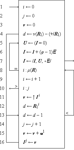 |
Legend | |||||||||||||||||||||
| Program 1.20
Determination of the index matrix I associated with a right list matrix R | ||||||||||||||||||||||
|
Program 1.20. In each execution of the main loop 13-16,
the ith row of the right list R
is examined to determine the index vector
of each node on the succeeding
level which is directly reachable from it.
The number of such nodes is controlled
by the parameter d,
initialized to the degree
of the ith node by step 12.
The (right list) index of the nodes reachable
from node i is determined by j,
which is incremented on step 14
as the index vector of each node is determined.
The index vectors of the successive nodes reachable
from node i have the final components
Since j is, at step 10,
equal to the current number of roots r augmented
by the cumulative degrees
of the first When step 5 is first reached, the index matrix I is complete but is expressed in 1-origin indexing with zeros representing the null elements. Steps 5-7 translate the matrix to the origin φ and mask in the necessary null elements. |
 |
Legend | |||||||||||||||||||||||||||
| Program 1.21
Determination of the index matrix I associated with a left list matrix L | ||||||||||||||||||||||||||||
|
Program 1.21.
The index vectors I j
are determined in order under control of the parameter.
The loop 5-18 traces a continuous path through the tree,
determining the index of each successive node
of the path by rotating the index of the
preceding node (step 17) and adding one
to the last component (step 13),
and maintaining in the connection vector c
a record ci+1
of the index j of the successor
of node i in the path traced.
The path is interrupted by the occurrence of a leaf
(that is,
|
Tree, path, and level compression
The tree compression
P ← U/T
specifies a tree P obtained from T
by suppressing those nodes corresponding
to zeros of the logical tree U,
and reconnecting so that for every
pair of nodes x, y of P,
x belongs to the subtree
of P rooted in y if and only if
x belongs to the subtree of T rooted in y.
If, for example, T is the tree
of Fig. 1.16
with n as the alphabet,
and U is the tree of Fig. 1.22a,
then P is the tree of Fig. 1.22b.
The new indices are shown to the left
of each node of P.
The set of nodes
U |
 |
U/T |
| Figure 1.22. Compression of tree T of Fig. 1.16 (with n = alphabet) | ||
The compress operation is best executed on the left list because of the grouping by subtrees. Program 1.23 gives a suitable algorithm which also serves as a formal definition of the compress operation.
 |
Legend | ||||||||||||||||||
| Program 1.23 Determination of the left list L = ⍺2/[(U/T) | |||||||||||||||||||
|
Program 1.23. The vector u is specified as the node vector of the left list of the controlling logical tree U and controls the subsequent process. Step 4 determines j as the index of the first zero component of u. Steps 6 and 7 then delete the corresponding nodes of u and of the left list of T, but only after step 5 has determined d as the change in degree which this deletion will occasion to the root of the smallest subtree containing the deleted node. Steps 9-11 perform a backward scan of the degree vector to determine j as the index of the root of the subtree, and step 12 effects the requisite change in its degree. The exit on step 9 occurs only if the node deleted is a root of the original tree, in which event no change is produced in the degree of any other node. |
Two further compress operations controlled by logical vectors are defined as follows. Path compression is denoted by
P ← u/T.
P is obtained from T
by suppressing every node on level j
if
P ← u//T,
and P is obtained from T
by deleting each rooted subtree
Ti for which
Path compression by a unit vector ∊ j produces a tree of height one. Such a tree is, in effect, a vector and will be treated as one.
Two related special logical trees are defined:
the path tree
uE
such that
/ uE
= 0//uE
= 0,
Extension of other operations to trees
Two trees are compatible if they have the same structure. Elementary binary operations are extended node by node to compatible trees. For example,
Z ← X × Y
implies that node i of Z is the product of node i of X and node i of Y for all i. Similarly,
M ← b ⍳ j T
specifies M as a tree (of the same structure as T) such that node i of M is the j-origin b-index of node i of T.
The mapping operation is extended to trees so as to permute the rooted subtrees of a tree. Formally
P ← m ∫j T
implies that
Permutation of the subtrees rooted in node i of T can be effected as follows:
1/Ti
← m ∫
(1/Ti)
The notation //T
will denote the application of the binary operator
or relation
to the nodes of T in right list order
(i.e., down successive levels)
and /T
will denote the same application in left list order
(i.e., across paths).
If the operator is symmetric
(i.e., its operands commute), then
//T =
/T
Maximization (U⌈T) and minimization (U⌊T) are extended to trees in the obvious way.
| ||||||||||
Figure 1.24. Set selection and maximum prefix and suffix operations | ||||||||||


 ⍺//U
⍺//U
 ⍵//U
⍵//U
 σ//U
σ//U
 τ//U
τ//UThe operations ⍺/u, ⍵/u, σ/u, and τ/u are each extended in two ways: across paths and down levels. Examples of each appear in Fig. 1.24. Operations extending down levels are denoted by double virgules and represent an application of the corresponding vector operation to each level of the tree considered as a vector. For example, the statement
V ← σ//A
implies that each level of V
is the forward set selection
of the corresponding level of A,
that is,
V ← ⍺/U
implies that V is obtained from the logical tree U by setting to zero all nodes of any subtree rooted in a zero node, and
V ← ⍵/U
implies that V is obtained from U by setting to zero every node whose subtree contains a zero node. The definitions of σ/U and τ/U are analogous.
Homogeneous trees
If, for all j,
every node on level j
of a tree T is either of degree zero or of
degree ν j+1(T),
then the tree T is said to be uniform.
If all leaves of a uniform tree T lie
in the same level (necessarily the top),
then the tree is said to be homogeneous.
The structure of a homogeneous tree
is completely characterized
by its dispersion vector ν(T)).
All maximal paths in a homogeneous
tree are clearly of the same length, namely
 | ||||||
| Figure 1.25. Homogeneous tree H and dispersion and moment vectors |
A tree T for which
1/ν(T)
= m∊
The jth component of the moment vector
of a homogeneous tree is clearly equal to
the product of the first j components
of the dispersion vector, that is,
+ I)
ν(T)).
Tree compression of a homogeneous tree H
(that is, U/H)
does not generally produce a homogeneous tree,
and, in fact, any tree P of
arbitrary structure can be represented
by a pair of homogeneous trees U and H
such that )⍺1.
Since the structure of a homogeneous tree is completely specified by its dispersion vector k, the structure of the special logical trees can be specified in the forms E(k), uE(k), and uE(k).
In a homogeneous tree, the right list or left list index of a node can be determined as an explicit function of its index vector. Conversely, the index vector i can be determined directly from the corresponding left list index, to be denoted by l(i), or from the right list index r(i). In developing the relations between indices it will be convenient to use 0-origin indexing throughout.
The right list index is given by
r(i) = f(i) + g(i),
where
f(i)
= +/⍺ν(i)–1/μ(T)
is the number of nodes in the first
g(i) = (⍺ν(i)/ν(T)) ⊥ i
is the rank of node i
in the ν(i)th level.
For example, if
Since f(i) depends only on ν(i),
the index i may be determined
from r by first determining ν(i)
as the largest value for which
(⍺ν(i)/ν(T)) ⊥ i = r – f(i).
In tracing a path through a tree,
the kth node of the set reachable from
node i is the node
(k).
| f(j) = f(i) + (μ(T))ν(i)–1, | |
| g(j) = g(i) × (ν(T))ν(i) + jν–1. |
In the special case of a singular homogeneous m-way tree,
| f(i) | = | 1+ m + m2 + … + mν(i)–2 | ||
| = | (m∊) ⊥ ∊(ν(i) – 1) | |||
| = |
| |||

Hence
r(j) = m × r(i) + 1 + jν–1.
The left list index l(i)
is most conveniently expressed as a function of
ν(i) and
of the vector z(i)
(zero extension of i),
where
The zero extension has the obvious property
that every node above the
path T z(i)
precedes node i in the left list,
and every node below the path follows it.
The number of nodes in the path which precede node i
is
The number of leaves above the path
T z(i) is
l(i) =
ν(i) – 1 +  (⍺ j/ν(T))
⊥ (⍺ j/z(i)).
(⍺ j/ν(T))
⊥ (⍺ j/z(i)).
For example, if
l(i) = z(i),
where
z(i) = 10.
z = l + 1 –
ν(i),
z(i).
References
| • | Birkhoff, G., and S. MacLane (1941), A Survey of Modern Algebra, Macmillian, New York. |
| • | Burks, A.W., D.W. Warren, and J.B. Wright (1954), “An Analysis of a Logical Machine Using Parenthesis-free Notation”, Mathematical Tables and Other Aids to Computation, vol. VIII, pp. 53-57. |
| • | Dickson, L.E. (1939), New First Course in the Theory of Equations, Wiley, New York. |
| • | Garner, Harvey L. (1959), “The Residue Number System”, IRE Transactions, vol. EC-8, pp. 140-147. |
| • | Goldstine, H.H., and J. von Neumann (1947), “Planning and Coding of Problems for an Electronic Computing Instrument”, Report on the Mathematical and Logical Aspects of an Electronic Computing Instrument, Part II, vol. 1, Institute for Advanced Study, Princeton. |
| • | Iverson, K.E. (1954), “Machine Solutions of Linear Differential Equations”, Doctoral Thesis, Harvard University. |
| • | Jacobson, N. (1951), Lectures in Abstract Algebra, vol. 1, Van Nostrand, New York. |
| • | Kunz, K.S. (1957), Numerical Analysis, McGraw-Hill, New York. |
| • | Margenau, H., and G.M. Murphy (1943), The Mathematics of Physics and Chemistry, Van Nostrand, New York. |
| • | Phister, M. (1958), Logical Design of Digital Computers, Wiley, New York. |
| • | Richards, R.K. (1955), Arithmetic Operations in Digital Computers, Van Nostrand, New York. |
| • | Riordan, J. (1958), An Introduction to Combinatorial Analysis, Wiley, New York. |
| • | Rutishauser, H. (1959), “Zur Matrizeninversion nach Gauss-Jordan”, Zeitschrift für Angewandte Mathematik und Physik, vol. X, pp. 281-291. |
| • | Wright, H.N. (1939), First Course in Theory of Numbers, Wiley, New York. |
Notes
 .
Moreover,
.
Moreover,  .
The remaining two transformations can be
denoted by
.
The remaining two transformations can be
denoted by  and
and
 ,
with the convention that the operator nearest
the operand (i.e., the horizontal)
is executed first.
,
with the convention that the operator nearest
the operand (i.e., the horizontal)
is executed first.
Exercises
Organize each of the programs according to the method of leading decisions. Except where otherwise indicated, use 1-origin indexing. The conventions of Sec. S.1 of the Summary of Notation will be used in the statement of each of the exercises.
1.1 Let
| (a) | the dimensions ν(d), ν(s), and ν(x). | |
| (b) | the vectors x + y, x – y, x × y, x ÷ y, and u + v. | |
| (c) | the logical vectors u ∧ v, u ∨ v, (u ≠ v), and (u = v). | |
| (d) | the reductions +/x, ×/y, ∧/u, and ∨/v. | |
| (e) | the base two values of u and of v, that is, +/(x × u), and +/(x × v). | |
| (f) | the rotated vectors 2 ↓ d, 4 ↑ s, and ↑ y. | |
| (g) | the unit vectors ∊1(5) in a 1-origin system, and ∊2(5) in a 0-origin system. | |
| (f) | the infixes (⍺5(7) ∧ ⍵5(7)) and 2 ↓ ⍺3(7). |
1.2 Show that
| (a) | ×/⍳1(n) = n! (Include the case n = 0.) | |
| (b) | +/⍳ j(n) = n(n + 2j – 1) ÷ 2. | |
| (c) | ×/(k ↑ x) = ×/x. | |
| (d) | (k ↑ x) + (k ↑ y) = k ↑ (x + y). |
1.3 Write detailed (i.e., component-by-component) programs for the following operations. Include tests for compatibility of the operands.
|
|
1.4 Established the identities
| (a) | /a, u, b/
= \/a, u, u/b\. | |
| (b) | \a, u, b\
= /\a, u, u\b/. |
1.5 The classic “rings-o-seven” puzzle can be posed as follows: an order collection of n rings is to be placed on (removed from) a bar under the following constraints:
| (i) | ring n may be placed on or removed at will. | |
| (ii) | ring k may be placed on or removed only if ring (k + 1) is on and all succeeding rings are off. |
| (a) | u = ∊ [The successive values of u represent a reflected Gray code; see Phister (1958).] | |
| (b) | u arbitrary. |
1.6 The ordered array of variables used to represent a variable x in some coding system may be considered as a vector representation of x, denoted by ⍴(x). In the 8421 code for decimal digits, for example, ⍴(0) = (0, 0, 0, 0), ⍴(1) = (0, 0, 0, 1), and, in general, ⍴(x) is defined by the relation +/[w × ⍴(x)] = x, where w = (8, 4, 2, 1). For each of the following coding systems, (see Richards, pp. 183-184 for definitions), write a concise expression for ⍴(x):
| (a) | the excess-three code for decimal digits. | |
| (b) | any chosen two-out-of-five code. | |
| (c) | any chosen biquinary code. | |
| (d) | the semaphore code for the alphabet (see any good dictionary). Denote each code by a two-component vector ⍴(x) ⊆ ⍳0(8). Use a⍳x, where a = (a, b, c, …, z). |
1.7 Let X be a square sparse matrix
represented by the logical matrix U = (X ≠ 0)
and either or both the vectors
r = U/X, and
c = U//X.
Write programs to determine the product
Y = X X,
using the arguments
| (a) | r, c, and U. | |
| (b) | r and U. | |
| (c) | c and U. |
1.8 Prove that
| (a) | ⌈x⌉ = –⌊–x⌋ | |
| (b) | ⌊⌊ a ÷ b⌋ ÷ c⌋ = ⌊ a ÷ bc⌋ for all positive integers a, b, and c. |
1.9 Let r = E/A, and c = E//A be the row list and column list, respectively, of the matrix A, and let r h, Aji, and ck be the corresponding elements of the three representations of A. Determine:
| (a) | h as a function of k, ν(A), and μ(A). | |
| (b) | k as a function of h, ν(A), and μ(A). | |
| (c) | the permutation vector h such that c = h ∫ r. |
1.10 Show that
| (a) |
∧/u = | |
| (b) | ≠/u = 2|0 +/u (Use induction.) | |
| (c) |
=/u = | |
| (d) |
≠/u = | |
| (e) |
U v =
(2∊) |0
(U v).
| |
| (f) |
U V =
| |
| (g) |
(t u) ∧
(v w) =
(t w) ∧
(v u).
|
1.11
| (a) |
Show that +/x =
+/(/x)
+(u/x).
(Include the case u = 0.)
| |
| (b) |
What properties are required of an operator
that it satisfy the relation
established for + in part (a)?
|
1.12 Show that
| (a) |
X Y =
(/X)
(//Y) +
(u/X)
(u//Y).
| |
| (b) |
u/(X Y)
= X
(u/Y).
| |
| (c) |
u//(X Y)
= (u//X)
Y.
| |
| (d) | (u ∧ v)/a = (u/v)/(u/a). |
1.13 Use the result of Exercise 1.11 (b) to extend the results of Exercise 1.12 (a-c) to logical operators.
1.14 Write programs to determine:
| (a) | the value of the polynomial x at the point a, that is, to evaluate (y∊) ⊥ x for y = a. Use no more than ν(x) multiplications. | |
| (b) |
the derivative of the polynomial x,
that is, the vector z such that (y∊) ⊥ z =  ((y∊) ⊥ x),
and ν(z) = ν(x).
((y∊) ⊥ x),
and ν(z) = ν(x).
| |
| (c) |
the integral z of the polynomial x
satisfying the boundary condition (a∊) ⊥ z = b. | |
| (d) | the quotient q and remainder r obtained in dividing the polynomial n by the polynomial d, for ν(d) ≤ ν(n). | |
| (e) | the value of the polynomial n at the point a by using part (d) with d = (1, –a). | |
| (f) |
the value of
((y∊) ⊥ n)
at the point a by two applications of part (e).
| |
| (g) | an approximate real root of the equation (y∊) ⊥ x = 0 using parts (e) and (f) and the Newton-Raphson formula [Kunz (1957)]. |
1.15 Let the components of the vector r be the real roots of a polynomial x. Write a program to
| (a) | determine the symmetric functions of r. [Dickson (1939), Ch. X.] | |
| (b) | determine x as a function of r. |
1.16 Write a program to determine the polynomial x consisting of the first n terms of the exponential series 1 + y + y²/2! + … .
1.17 Write a program to determine the moduli of all roots of the polynomial x, using the Graeffe method [Kunz (1957)]. Assume that operations for the logarithm and exponential functions are available as subroutines.
1.18 List all the 1-origin permutation vectors of dimension four which are self-inverse.
1.19 Using 1-origin indexing, write programs to derive
| (a) | the permutation k which is inverse to the permutation j. | |
| (b) | a permutation j which transforms a given logical vector u to a prefix vector. |
1.20 A square logical matrix U such that +/U = +//U = ∊ is sometimes called a permutation matrix, since premultiplication of a numerical vector x determines a permutation of x. Write programs to determine
| (a) |
the permutation matrix U corresponding
to the 1-origin permutation vector k,
that is, determine U such that
U x =
k ∫1 x.
| |
| (b) | the permutation k corresponding to a given permutation matrix U. | |
| (c) | the permutation V which is inverse to the permutation U. |
1.21 Let p be the vector representation
of a permutation and let c be the standard representation
in terms of disjoint cycles, including all cycles of one
[Jacobson (1951), p. 34].
Each cycle of c is enclosed in square brackets,
each half-bracket being considered as a component of c.
For example, c =
| (a) | Write a program to determine p as a function of a well formed permutation c. Include determination of the dimension of p. | |
| (b) | Modify the program in part (a) to incorporate checks on the well formation of c. If c is ill formed, the vector p is to be defined as the literal “ill formed”. | |
| (c) |
Modify part (b) to process a sequence of vectors
c1, c2, …,
each pair being separated by a single null element,
and the end of the sequence being indicated by a pair
of successive null elements, i.e., to process
z = c1
(∘)
c2
…
c r
(∘,∘).
Include checks on the well formation
of each permutation.
| |
| (d) | Write a program to determine the parity [Jacobson (1951), p. 36] of a permutation vector p. |
1.22 Write detailed programs for the following processes:
|
|
1.23
| (a) | Copy onto file Φ12 successive groups of items from the row of files Φ⍳ in cyclic order, omitting any exhausted files. The end of each group is demarked by a partition λ2, and the end of each file by a partition λ3. | |
| (b) | A file which is always recorded in the forward direction and read in the backward direction functions as a stack. Using file Φ22 as a stack, modify the program of part (a) so as to reverse (in the output file Φ12) the order of the items within each group. |
1.24 The accompanying node vector n and connecting matrix C together specify a directed graph (C j i = 1 indicates a branch from node i to node j) which is, in fact, a tree.
n = (a, b, c, d, e, f, g)
| C = |  |
0 0 0 0 1 1 0 |  |
| 0 0 0 0 0 0 0 | |||
| 1 0 0 1 0 0 0 | |||
| 0 0 0 0 0 0 0 | |||
| 0 0 0 0 0 0 0 | |||
| 0 0 0 0 0 0 0 | |||
| 0 1 0 0 0 0 0 |
| (a) | Draw one of the possible ordered trees represented by n and C. | |
| (b) | For the tree T of part (a) show the full left list [T. | |
| (c) | Show the full right list ]T. |
1.25 Write programs which includes tests on compatibility and which determine
| (a) | L = [T from R = ]T | |
| (b) | S = ](u/T) from μ(T), ]T, and u | |
| (c) | M = [(u//T) from L = [T and u | |
| (d) | M = [(k ∫1 T) from L = [T and k |
1.26
| (a) | Give an example of a well formed right list which demonstrates that a prefix of a right list is not, in general, well formed. | |
| (b) | Show clearly where the argument used in establishing the well formation of any suffix of a well formed list breaks down when applied to a prefix. |
1.27 Give formal proofs for the facts that
| (a) | a left list groups nodes by subtrees. | |
| (b) | a right list groups nodes by levels. | |
| (c) | μ1(T) = ν(d) – +/d, where d is the degree vector of T. |
1.28 Write programs to determine μ(T) as a function of
| (a) | the left list degree vector of T. | |
| (b) | the right list degree vector of T. |
1.29 Trace Programs 1.20 and 1.21 for the tree of Exercise 1.24.
1.30 Show that for a homogeneous tree H,
μ(H) = y ⊥ y,
where  = ν(H).
1.31 If H is homogeneous, ν(H) = (3, 2, 3, 4), and i = (1, 0, 2), determine, in a 0-origin system
| (a) | the left list index l(i). | |
| (b) | the right list index r(i). | |
| (c) | the index j of the node whose left list index is 27. |
1.32
| (a) |
If K = ⍳0(n)
↓ (∊(n)
⍳0(n)),
show that K +
 =
n(E –
I). =
n(E –
I).
| |
| (b) |
If y is any permutation of x
and ν(x) = n, show that
x K
x =
y K
y.
|
1.33 Using the Euclidean algorithm, write programs to determine:
| (a) | d as the greatest common divisor of positive integers x and y. | |
| (b) | d as the g.c.d. of x and y, where d, x, and y represent polynomials in z (e.g., ((z∊) ⊥ x). |
1.34 To assure uniqueness, the number of different digits (symbols) used in a base b number system must not exceed b. The limitation to the particular range 0 ≤ a i < b is, however, not essential. For example, a base three system can be constructed using digits –1, 0, and 1, for which it is convenient to adopt the symbols –, 0, and +, respectively. The positive numbers beginning at zero are then represented by the sequence 0, +, + –, +0, + +, + – –, + –0, + – +, + 0 –, +00, etc. The negative numbers beginning at 0 are 0, –, – +, –0, – –, – + +, – +0, – + –, –0 +, –00, etc.
| (a) | Construct addition and multiplication tables for this number system and calculate the sum and the product of the numbers 0 – and – –. Use the decimal system to check all results. | |
| (b) | Negative numbers are represented in this system without the attachment of a special sign position. Special rules regarding sing are therefore banished except that it is necesssary to formulate a rule for changing the sign of a number, i.e. to multiply by minus one. Formulate such a rule. |
1.35 For any integer n, let x2 = 2 |0 n, x3 = 3 |0 n, x5 = 5 |0 n, and x7 = 7 |0 n. As shown by Garner (1959), the ordered array (x2, x3, x5, x7) provides a representation of the integer n in a so-called residue number system.
| (a) | Write the residue representations of the first ten nonnegative integers. | |||||||
| (b) |
For integers n in the range 0 ≤ n <
(2 × 3 × 5 × 7) show:
| |||||||
| (c) | Discuss the choice of moduli for extending the range of the representation. | |||||||
| (d) | Show that the algorithm derived in part (b) is valid for all positive and negative integers in the range –a/2 ≤ n < a/2 for a = 2 × 3 × 5 × 7. | |||||||
| (e) | Derive an algorithm for obtaining –n from n. | |||||||
| (f) | Derive an algorithm for multiplication. | |||||||
| (g) | The sign of the number (i.e., its relation to zero) is not displayed directly by this representation. Convince yourself that its determination is nontrivial. |
1.36 Let x, y, and z be the positional representations of the numbers x, y, and z respectively. Using the floor and residue operations, write programs to determine z as a function of x and y, where z = x + y and the representation in use is
| (a) | base b. | |
| (b) | mixed base b. | |
| (c) | the +, –, 0 base three system (of Exercise 1.34). | |
| (d) | the residue number system (of Exercise 1.35). |
1.37 Write programs for the multiplication z = x × y for each of the cases of Exercise 1.36.
1.38 Write programs to convert in each direction between the following pairs of number systems:
| (a) | base b1 and b2. | |
| (b) | base b1 and b2. | |
| (c) | base three and the +, –, 0 base three of Exercise 1.34. | |
| (d) | residue and base b (Exercise 1.35). |
1.39
| (a) |
Show that the superdiagonal matrices satisfy
jI
kI =
(j+k)I.
| |
| (b) | A matrix of the form J = (xI + 1I) is called a Jordan box. Write the expansion of the nth power of J. | |
| (c) |
Show that
X Y =
X1 Y1 +
X2 Y2 +
… +
Xν(X)
Y ν(X).
| |
| (d) |
Determine an explicit solution
to the set of linear equations
A x = y,
where u/x = a
and v/y = b
are known and where +/u + +/v
= ν(A) = &mu(A).
State the conditions for the existence
of a unique solution.
|
1.40 Any nonsingular matrix A
can be reduced to the identity I
by a sequence of row operations of the form
Ai ←
xAi +
yAi, or
Ai ← A j.
The process which accomplishes this
(using row operations only) by reducing successive column
vectors to the successive unit vectors is called
Jordan or complete elimination.
If the same sequence of row operations is executed
upon the identity matrix,
it will be transformed to the matrix B
such that B
A = I.
The inverse of A can therefore be obtained
by performing Jordan elimination on the matrix
M = A
I
so as to reduce the first ν(A) columns
to the identity.
The last ν(A) columns
are then the inverse of A.
| (a) | Write a program to determine the inverse of A by Jordan elimination. | |
| (b) | The sequence of operations which reduce the ith column of A to ∊i is called the ith step of the process, and the ith diagonal element at the beginning of the ith step is called the ith pivot element. Modify the program of part (a) so that each step is preceded by a column permutation which yields the largest (in absolute value) pivot element possible. This modification tends to reduce the accumulation of round-off errors. | |
| (c) | In the Jordan elimination of part (a), it is unnecessary to store the identity matrix explicitly, and, since the ith column is first affected at the ith step, only one new column need be brought in at each step. Moreover, the ith column of A may be discarded after its reduction to ∊i on the ith step, and it is therefore necessary to store only a square matrix at all times. Show that by shifting all columns to the left and by moving the rows upward cyclically, a very uniform process results, with the pivot element in the leading position at every step [Iverson (1954) or Rutishauser (1959)]. Write a program for the process. | |
| (d) | Modify part (c) to allow the choice of pivot elements as in part (b). The effects of the permutation on the not explicitly recorded identity cannot be indicated directly, but the performance of the same set of permutations in reverse order upon the rows of the resulting inverse produces the same result. Verify this and program the process. |
1.41
| (a) | Show that a group [Jacobson (1951)] can be represented by a square matrix M such that each row and each column is a permutation vector. | |
| (b) | Show that M i = Mi = ⍳1 for some i. | |
| (c) | What are the necessary and sufficient conditions that the group represented by M be Abelian? | |
| (d) | What a program to determine all cyclic subgroups of a group represented by M. |
1.42 If U is a logical matrix whose rows are each nonzero, mutually disjoint, and collectively exhaustive (that is, (+/U ≥ ∊) = ∊, and +//U = ∊), then U defines an m-way partition of n, where m = μ(U), and n = ν(U). The partition is more commonly represented by the vector p = +/U [Riordan (1958), p. 107]. Clearly +/p = n. Write a program to generate
| (a) | all partitions U of a given integer n. | |
| (b) | all distinct partitions of n, where U and V are considered equivalent if p = +/U is a permutation of q = +/V. |
1.43 Let = x be a space vector
(i.e., of dimension three), and let R(x)
be the square matrix
⍳ ↑ (∊
x). Show that
| (a) |
+/R(x × y) =
(x
y) × ∊
| |
| (b) |
∊
(x × y) =
x y
| |
| (c) |
(+/R(x × y))
(w × z) =
(x y) ×
(w z)
| |
| (d) |
(x y) ×
(x y) =
(x × y) +
(x × y) +
2(↓ x × ↑ y)
(↓ x × ↑ y).
|
1.44 Let x · y = (↑ x × ↓ y) – (↓ x × ↑ y) be the vector product of x and y for vectors of dimension three. Show that
| (a) | this agrees with the usual definition [Margenau and Murphy (1943)]. | |
| (b) | x · y = –(y · x) | |
| (c) |
x · y is perpendicular
to x, that is, x
(x · y) = 0.
(Use the fact that ↓ x = 2↑x
for a vector of dimension three.)
|
1.45 Let [x] =
 be the length of x,
and let x γ y =
be the length of x,
and let x γ y =
 be the cosine of the angle between
x and y,
and let x σ y
=
be the cosine of the angle between
x and y,
and let x σ y
=  be
the sine of the angle.
Use the results of Exercises 1.43 and 1.44
to show that for space vectors
be
the sine of the angle.
Use the results of Exercises 1.43 and 1.44
to show that for space vectors
| (a) | [x · y] = [x] × [y] × (x σ y). Note that [x · y] is the area enclosed by the parallelogram defined by x and y. | |
| (b) |
(x · y) · z
= (x z)
× y –
(y z)
× x
| |
| (c) |
(x · y)
z = x
(y · z).
|
Chapter 3 Representation of Variables
3.1 Allocation and encoding
Although the abstract description of a program may be presented in any suitable language, its automatic execution must be performed on some specified representation of the relevant operands. The specification of this representation presents two distinct aspects—allocation and encoding.
An allocation specifies the correspondences between physical devices and the variables represented thereby. An encoding specifies the correspondences between the distinct states of the physical devices and the literals which they represent. If, for example, certain numerical data are to be represented by a set of 50 two-state devices, the two-out-of-five coding system of Exercise 1.6 might be chosen, and it would then remain to specify the allocation. The two-digit quantity “hours worked” might be allocated as follows: devices 31-35 represent components 1-5, respectively, of the first digit, and devices 29, 16, 17, 24, and 47 represent components 1, 2, 3, 4, 5, respectively, of the second digit.
The encoding of a variable will be specified
by an encoding matrix C and
associated format vector f
such that the rows of  /C
list the representands
and the rows of f/C
list the corresponding representations.
The encoding is normally fixed and normally
concerns the programmer only in the
translation of input or output data.
Even this translation is usually
handled in a routine manner,
and attention will therefore be restricted
primarily to the problem of allocation.
/C
list the representands
and the rows of f/C
list the corresponding representations.
The encoding is normally fixed and normally
concerns the programmer only in the
translation of input or output data.
Even this translation is usually
handled in a routine manner,
and attention will therefore be restricted
primarily to the problem of allocation.
However, the encoding of numeric quantities warrants special comment. It includes the representation of the sign and of the scale, as well as the representation of the significant digits. Small numbers, such as indices, admit not only of the usual positional representation but also of the use of the unit vector ∊ j to represent the number j (i.e., a one-out-of-n coding system), or of the use of a logical vector of weight j (i.e., a base 1 number system).
Allocation will be described in terms of the physical vector π, which denotes the physical storage elements of the computer. Each component of π corresponds to one of the ν(π) similar physical devices available, its range of values is the set of physical states achievable by each device, and its index is the address of the device. Each component of π may correspond to a computer register, an individual character position in a register, or an individual binary digit within a character, depending on the degree of resolution appropriate to the allocation problem considered. The 0-origin indexing normally used for computer addresses will be used for the physical vector, but 1-origin indexing will, throughout this chapter, normally be employed for all other structured operands.
An index of the physical vector will be called an address and will itself be represented in the (perhaps mixed) radix appropriate to the given computer. The Univac, for example, employs base ten addressing for the registers, and (because of the use of 12-character words) a radix of twelve for finer resolution. The address of the fourth character of register 675 might therefore be written as 675.3. In computers which have two or more independent addressing systems (e.g., the independent addressing systems for main memory and for auxiliary storage in the IBM 705), superscripts may be used to identify the several physical vectors π j.
In general, the representation
of a quantity x is a vector
(to be denoted by ⍴(x))
whose components are chosen
from the physical vector π.
Thus ⍴(x) = k∫π,
where k is a mapping vector
associated with x.
The dimension of the representation
(that is, ν(⍴(x)))
is called the dimension of x in π.
If, for example, ⍴(x) =
3.2 Representation of structured operands
The grid matrix
If each component of a vector x
has a solid representation,
then the representation of the entire vector
is said to be solid and may be characterized
by the grid matrix Γ(x),
of dimension
| Γ(x) = |  |
17 2 |  |
. | |
| 19 4 | |||||
| 27 5 | |||||
| 23 1 | |||||
| 32 3 |
Any structured operand can first be reduced to an equivalent vector, and the grid matrix therefore suffices for describing the representation of any construct, providing only that the representation of each of its elements is solid. Thus a matrix X may be represented by either the row-by-row list r = E/X or the column-by-column list c = E//X, and a tree T may be represented by the left list matrix [T or the right list matrix ]T, either of which may be represented, in turn, by a vector.
If a process involves only a small number of variables, it is practical to make their allocation implicit in the algorithm, i.e., to incorporate in the algorithm the selection operations on the vector π necessary to extract the appropriate variables. This is the procedure usually employed, for example, in simple computer programs. In processes involving numerous variables, implicit allocation may become too cumbersome and confusing, and more systematic procedures are needed.
Figure 3.1

Figure 3.2 Linear Representation of a matrix X
Linear representations
The representation of a structured operand
is said to be linear
if each component is represented
by an infix of the form
A linear representation is solid and can clearly be characterized by a small number of parameters—the dimension d of each component and the coefficients in the linear expression l. The representation of a vector x is linear if and only if Γ2(x) = d∊ and the difference δ = Γ1i(x) – Γ1i–1(x) is constant for i = 2, 3, … , ν(x).
If l = p + qi + rj is the function defining a linear representation of a matrix x and if a is the leading address of a given element, then the leading address of the succeeding element in the row (or column) is simply a + r (or a + q). Frequently, the succession must be cyclic, and the resulting sum must be reduced modulo ν(x) × r (or μ(x) × q). The inherent convenience of linear representations is further enhanced by index registers, which provide efficient incrementation and comparison of addresses.
Linear representation of a structured operand requires that all components be of the same dimension in π. This common dimension may, however, be achieved by appending null elements to the shorter components. The convenience of the linear representation must then be weighed against the waste occasioned by the null elements. Moreover, if several vectors or matrices are to be represented and if each is of unspecified total dimension in π, it may be impossible to allot to each an infix sufficiently large to permit linear representation. Consequently, a linear representation is not always practicable.
Nonlinear representations
Since the use of the grid matrix imposes only the condition of solidity for each component, it permits an allocation which is sufficiently general for most purposes. The grid matrix serves in two distinct capacities: (1) as a useful conceptual device for describing an allocation even when the actual allocation is implicit in the program, and (2) as a parameter which enters directly into an algorithm and explicitly specifies the allocation.
If the grid matrix is used in a program as an explicit specification of the allocation, then the grid matrix must itself be represented by the physical vector. There remains, therefore, the problem of choosing a suitable allocation for the grid matrix itself; a linear allocation is illustrated by Fig.3.lb.
If the grid matrix Γ(x) itself employs a linear representation, its use offers advantages over the direct use of a linear representation of x only if the total dimension of Γ in π is much less than the total dimension of x in π when linear representations are employed for both. This is frequently the case, since each element of a grid matrix belongs to the index set of π (that is, to ⍳0(ν(π))), and the dimension of each element in π is therefore both uniform and relatively small. Program 3.3 shows the use of the grid matrix Γ(x) and the encoding matrix C in determining the kth component of the vector x.
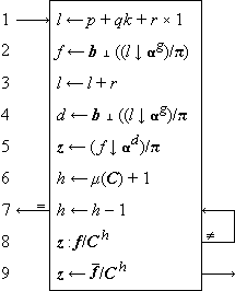 |
Legend |
||||||||||||||||||||||
Program 3.3 Determination of
z = ⍴(xk)
and z = xk
from a linear representation of the grid matrix
Γ(x)
|
Program 3.3. A linear representation is assumed
for Γ(x),
with element Γji(x)
represented by the infix
Steps 7-9 perform the decoding of z = ⍴(xk) to obtain z as the actual value of xk. Since this process is normally performed by human or mechanical means (e.g., a printer) outside the purview of the programmer, it is here expressed directly in terms of the encoding matrix C rather than in terms of its representation. The left-pointing exit on step 7 is followed only if z does not occur as an entry in the encoding matrix. |
The form chosen for the grid matrix is one of several possible. The two
columns could, for example, represent the leading and final addresses of
the corresponding representations or the dimensions and final addresses.
The present choice of leading address f and dimension d
is, however, the most convenient for use in conjunction
with the notation adopted for infixes;
the logical vector
Chained representations[a]
If a linear representation is used for a vector, then the deletion of a component (as in a compress operation) necessitates the moving (i.e., respecification) of the representations of each of the subsequent components. Similarly, mesh operations (insertion) and permutations necessitate extensive respecification. The use of a grid matrix Γ(x) obviates such respecification in x, since appropriate changes can instead be made in Γ(x), where they may be much simpler to effect. If, for example, x is the vector represented as in Fig. 3.1a, and z is a quantity of dimension six in π, then the mesh operation
| x ← \x, ∊3, z\ |
may be effected by specifying the physical infix (70 ↓ ⍺6)/π by ⍴(z) and by respecifying Γ(x) as follows:
| Γ(x) = | |
17 2 | |
. | |
| 19 4 | |||||
| 70 6 | |||||
| 27 5 | |||||
| 23 1 | |||||
| 32 3 |
However, if the representation of Γ(x) is itself linear, then insertions, deletions, and permutations in x will occasion changes in all components of Γ(x) whose indices are affected. The need for a linear representation of the grid matrix (and hence for all linear representations) can be obviated by the use of a chained representation defined as follows.
Consider a vector y,
each of whose components yk
has a solid representation
⍴(yk)
whose infixes
(g ↓ ⍺g)/⍴(yk)
and
⍺g/⍴(yk)
are, respectively,
the dimension
of ⍴(yk) in π
and the leading address of the representation of
the (cyclically) succeeding component of y
(both in a base b system),
and whose suffix
2g/⍴(yk)
is the representation of the kth component
of some vector x.
Then (the representation of) y
is called a chained representation of x.
In other words, the representation of y
incorporates its own grid matrix
(with the address column Γ1(y)
rotated upward by one place)
as well as the representation of the vector x.
For example, if g = 2, b = 10∊,
and x =
| ⍴(y1) = (π17, π18, π19, π20, π21, π22, π23) = (6, 8, 0, 7, 3, 6, 5), | |
| ⍴(y2) = (π68, π69, π70, π71, π72) = (2, 6, 0, 5, 7), | |
| and | |
| ⍴(y3) = (π26, π27, π28, π29, π30, π31) = (1, 7, 0, 6, 2, 4), |
is a suitable chained representation of x.
The parameters required in executing an algorithm on a chained representation y are g, the common dimension in π of the elements of the grid matrix Γ1(y); b, the base of the number system employed in their representation; and f and h, the leading address and index, respectively, of the representation of some one component of y. The parameters g and b are usually common to the entire set of chained representations in use. Program 3.4 illustrates the type of algorithm required to determine ⍴(xk) from a given chained representation of x.
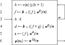 |
Legend |
Program 3.4 Determination of ⍴(xk) from a chained representation of x
|
Program 3.4. The loop (1-3) is executed ν(x)|0(k – h) times, with the result that at step 4 the parameter f is the leading address of ⍴(yk). Step 4 therefore specifies d as the dimension of ⍴(xk), that is, as the base b value of Γ2k(y). Step 5 then specifies z as ⍴(yk). Step 6 deletes those components of z which represent the elements of the grid matrix, leaving ⍴(xk). The parameters f and h are themselves respecified in the execution of the algorithm so that h becomes k and f becomes, appropriately, the leading address of ⍴(yk). A subsequent execution then begins from this new initial condition. |
The chained representation used thus far is cyclic
and contains no internal identification
of the first or the last components.
Such an identification can be incorporated
by adding a null component between the last
and first components of x.
Alternatively the identification may be achieved
without augmenting the dimension
but by sacrificing the end-around chaining,
i.e., by replacing the last component
of
The number of components
of a chained representation scanned
(steps 1-3 of Program 3.4)
in selecting the kth component of x
is given by
A vector x which is respecified only
by either deleting the final component
or by adding a new final component
(i.e., by operations of the form
 1/x, (z))
A simple example of the use of a chained stack occurs in representing the available (i.e., unused) segments of the physical vector π. This will be illustrated by a program for the vector compression
x ← v/x
executed on a forward-chained representation
of x.
The unused segments
representing the components
of /x
are returned to a backward-chained
stack or pool of available components.
A linear representation can usually
be used for logical control vectors such as v;
in any case the problems involved in their representation
are relatively trivial and will be subordinated
by expressing each operation directly in terms
of the logical vectors and not in terms
of the physical components representing them.
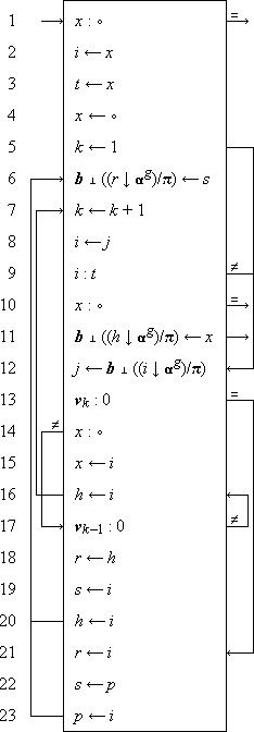 |
Legend |
Program 3.5
Program for x ← v/x
on a forward chained representation of x
and a backward chained stack of available segments
|
Program 3.5. In the major loop (6-23), k determines the index of the current component vk, and i and j determine the leading addresses of ⍴(xk) and ⍴(xk+1), respectively. These three parameters are cycled through successive values by steps 7, 8, and 12 and are initialized by steps 2,5, and 12. If vk = 0, the infix ⍴(xk) is returned to the pool by steps 21, 22, 23, and 6 so as to construct a backward chain. The parameter x specifies the leading address of ⍴(x1) unless ν(x) = 0, in which case x is null. Step 1 terminates the process if ν(x) = 0, and otherwise step 4 respecifies x as the null element. If v = 0, this null value of x remains; if not, the first nonzero component of v causes a branch to step 14. Since x = ∘, step 15 is executed to respecify x as the leading address of ⍴((v/x)1). Step 16 then specifies h, the leading address of the last completed component of v/x. Step 15 is never again executed. Components of v/x other than the first must each be chained (in a forward chain) to the preceding one. Hence the leading address i of a newly added component must be inserted in the last preceding component (whose leading address is h). This is normally done by steps 18, 19, and 6; step 20 respecifies h. If, however, the component xk–1 were also included, it would appear as the last completed component of v/x and would already be chained to the new component xk. This situation is recognized by step 17 and occasions a branch to step 16. Step 16 then respecifies h and repeats the loop without executing steps 18, 19, and 6. The process terminates when the cycle through the chained representation of x is completed, that is, when i returns to the original value of x, preserved as t by step 3. Step 10 is then executed, terminating the process directly if ν(v/x) = 0. Otherwise, step 11 is executed to close the chain of v/x, that is, to insert x, the leading address of ⍴((v/x)1), in the representation of the last component of v/x. |
A chained representation can be generalized to allow the direct representation of more complex constructs, such as trees, by incorporating the address of each of the successor components associated with a given component. This notion is formalized in the chain list matrix of Sec. 3.4. The same scheme can also be employed to produce an efficient combined representation of two or more vectors which share certain common components. If, for example, xj = xk, and chained representations are used for both x and z, then x may be represented in standard form except that component xj incorporates a secondary address, which is the leading address of zk+1. Moreover z has a standard representation except that zk–1 is chained to xj with an indicator to show that the secondary address of the succeeding component is to be used. Deletion of any vector component in such a shared system must occasion only the corresponding change in the address chain of the vector, the actual representation of the component being deleted only when no associated address remains.
Partitions
If the set a is the range of the components of the physical vector π, and if some element, say a1 is reserved as a partition symbol and is excluded from use in the normal representation of quantities, it can be inserted to demark the end (or beginning) of an infix of π. If the vector y is represented by a single infix of π such that the beginning of component yj+1 follows immediately after the terminal partition of yj, then the structure of y is completely represented by the partitions, and y is called a partitioned representation. A partitioned representation can be used for more complex operands, such as matrices, if a set of two or more distinct partition symbols are provided, one for each level of structure. The distinct partition symbols can, of course, be represented by multiple occurrences of a single symbol a1 rather than by distinct members of a.
A partitioned representation is similar to a double-chained representation without end-around chaining in the following particular: beginning from component yi, the component yj can be reached only by scanning all intervening components between i and j in increasing or decreasing order according as i < j or i > j. The file notation introduced in Sec. 1.22 clearly provides the operations appropriate to a partitioned representation of a vector, with conventions which suppress all inessential references to the partitions themselves.
The use of a partition to demark
the end of an infix is particularly convenient
when the infix must be processed component by component
for other reasons,
as in the use of magnetic tape or other serial storage.
The partition also appears to be more economical than
the grid matrix, which it replaces.
This apparent economy is, however, somewhat illusory,
since the reservation of a special partition symbol
reduces the information content of each nonpartition component
by the factor
Partitions can be employed in chained representations.
For example, the dimension in π
of each component of a chained representation y can be
specified implicitly by terminal partitions
instead of explicitly by the vector
Γ2(y)
of the grid matrix.
Thus if the elements of
Γ1(y) are of dimension g
in π, then
⍵1/⍴(yj) =
a1,
and
g ∧
1)/⍴(yj) =
⍴(xj),
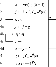 |
Legend |
Program 3.6 Determination of
⍴(xk)
from a chained representation of x
with terminal partitions a1
|
Program 3.6. The program is similar to Program 3.4 and the step numbering indicates the correspondences. The dimension d is so determined (steps 4a-d) as to exclude the terminal partition itself from the quantity z specified by step 5. Since only the first column of the grid matrix is incorporated in the partitioned representation, step 6 excises a prefix of dimension g rather than 2g as in Program 3.4. |
Pools
Components of the physical vector π in use for the representation of one quantity must not be allocated to the representation of some other quantity. The construction of a chained representation therefore poses one problem not encountered in its use, namely, the specification and observation of restrictions on the availability of components of π. The restrictions can conveniently be specified as a pool, consisting of the available components of π. Each allocation made must then be reflected in a corresponding change in the pool. Moreover, as each piece of data is deleted, the components allocated to it are returned to the pool.
If, as in Program 3.5, a pool is treated as a stack, then the component next taken from the pool is the component last added to it. The queue of components in the pool thus obeys a so-called last in first out, or LIFO discipline. The dimension in π of the last component of a pool will not, in general, agree with the dimension required for the next quantity it is called on to represent. If it exceeds the requirements, the extra segment may be left in the pool, and the pool therefore tends to accrue more and more components of smaller and smaller dimension. Hence it may be wise, or even essential, to revise the pool occasionally so as to coalesce the segments into the smallest possible number of infixes. This process can even be extended to allow substitutions in other vectors in order to return to the pool short segments which may unite existing segments of the pool. This, however, will require a systematic scan of the chained vectors.
If the dimension of the last component (or perhaps of all components) of the pool falls short of the requirements for representing a new quantity, segments of the pool can be chained together. This requires the use of a special partition symbol or other indication to distinguish two types of links, one which marks the end of a given representation and one which does not. More generally, it may be convenient to use multilevel partition symbols to distinguish several levels of links, as was suggested for the representation of a matrix.
Queue disciplines other than LIFO may be used. Three other types of primary interest in allocation queues are the FIFO (first in first out), the dimension-ordered, and the address-ordered disciplines. FIFO uses a forward chain and may be preferred over LIFO because it uses the entire original pool before using any returned (and usually shorter) segments.
The components of a dimension-ordered pool are maintained in ascending (or descending) order on their dimensions in π. This arrangement is convenient in selecting a pool element according to the dimension required. The components of an address-ordered pool are arranged in ascending order on their leading addresses. This arrangement facilitates the fusion of components which together form an infix of π.
If each of the available components of π is set to a special value which is used for no other purpose, then the available components can be determined by a scan of π. Such a pool has no structure imposed by chaining and will be called a marked pool.
A marked pool requires little maintenance, since components returned to it are simply marked, but selection from it requires a scan of π and is therefore relatively slow. The use of marked and chained pools may also be combined—all returned components go to a marked pool which is left undisturbed until the chained pool is exhausted, at which time the entire marked pool is organized into a chained pool.
Summary
Since any structured operand can first be reduced to an equivalent vector, the problems of representation can be discussed in terms of vectors alone. The characteristics of the linear, chained, and partitioned representations of a vector may be summarized as follows. A linear representation permits the address of any component to be computed directly as a linear function of its indices and hence requires no scanning of the vector. However, the strict limitations which it imposes on allocation may engender: (1) conflicts with allocations for other operands, (2) waste of storage due to the imposition of a common dimension in π for all components, or (3) uneconomical execution due to the extensive reallocations occasioned by the insertion or deletion of other than terminal components.
The concept of the grid matrix is helpful even when the corresponding allocation is implicit in the program. The explicit use of a grid matrix which is itself in a linear representation removes the restrictions on the allocation of the vector itself while retaining the advantage of direct address computation. The address computation differs from the linear case only in the addition of a single reference to the grid matrix and hence requires no scanning. The difficulties enumerated for the direct linear representation are not eliminated but merely shifted to the linearly represented grid matrix itself, where they may, however, prove much less serious.
A chained representation allows virtually arbitrary allocation, relatively simple operations for the insertion and deletion of components, the direct representation of more complex structures such as trees, and economical joint representations of vectors which have one or more components in common. However, a chained representation requires extra storage for the grid matrix which it incorporates and occasions additional operations for scanning when the components are selected in other than serial order. The required scanning can be reduced by the retention of auxiliary information which allows the chained representation to be entered at several points.
A partitioned representation requires the allocation of a single infix of π, and selection requires a fine scan, i.e., a component-by-component scan of π to detect partition symbols. Partitioning removes the need to incorporate the grid matrix explicitly and does not impose a common dimension in π for all components.
Mixed systems employing combinations
of linear, chained, and partitioned
representations are frequently advantageous.
Block chaining, for example,
involves the chaining of blocks,
each consisting of an infix of π
and each serving as a linear representation
of some infix of the represented vector.
Alternatively, each chained block may be
a partitioned representation of some infix.
3.3 Representation of matrices
Structured operands other than vectors
may be represented by first
reducing them to equivalent vectors which can,
by employing the techniques of the preceding section,
be represented, in turn, in the physical vector π.
In the case of a matrix A,
two alternative reductions are of interest,
the row list
A2 …
Aμ
| h = vi + j, | |
| k = i + μj. | |
| Consequently, | |
| i = ⌊h ÷ ν⌋ = μ |0 k, | |
| and | j = ν |0 h = ⌊k ÷ μ⌋. |
The dependence of h on k can be obtained directly by substituting the foregoing expressions in the identity
| h = ν × ⌊h ÷ ν⌋ + ν |0 h | |
| to yield | h = ν × (μ |0 k) + ⌊k ÷ μ⌋. |
| Similarly, | k = μ × (ν |0 h) + ⌊h ÷ ν⌋. |
The permutation h which carries the row list r into the column list c (that is, c = h∫0r) can be obtained directly from the foregoing expression for h as follows:
| h = ν × (μ∊ |0 ⍳0) + ⌊⍳0 ÷ μ∊⌋. |
The expression for the kth component
of h is identical with the expression
for h above.
Hence, if
If the row list (or column list) is itself represented linearly, then the address of any component Aji is obtained as a linear function of the indices i and j. If either a file or a chained representation is to be used for the list vector, then the components are processed most efficiently in serial order, and the use of column list or row list is dictated by the particular processes to be effected.
If a large proportion of the elements
of a matrix are null elements,
it is called a sparse matrix.
Sparse matrices occur frequently in numerical work
(where zero serves as the null element),
particularly in the treatment
of partial difference equations.
A sparse matrix A can be represented
compactly by the row list
r = U/A,
and the logical matrix U, where
U =
Alternatively, the column list
Let L be a matrix such that L1 is a list of the nonzero elements of a matrix A in arbitrary order, L2i is the column index in A of element L1i, and L3i is the row index in L of the next nonzero element following L1i in its row of A. If L1i is the last nonzero element in its row, L3i = ∘. Let fj be the row index in L of the first nonzero element of row Aj, and let fj = ∘ if Aj = 0. The following example shows corresponding values of f, L, and f :
|
|
|
The matrix L will be called a row-chained representation of A and may be used, together with the vector f, for the efficient scanning of any row Ai as illustrated by Program 3.7. The vector L3 can be modified so as to give the address in π directly rather than the row index in L of the next element in the row, and Program 3.7 can then be easily re-expressed in terms of the physical vector π.
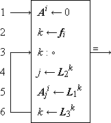 |
Legend |
Program 3.7 Determination of the row vector
Ai
from a row-chained representation of A
|
Program 3.7. Step 2 yields the index in L of the first element of the ith row of A. Step 4 determines its column index j, and step 6 determines the index of the succeeding component. The process terminates at step 3 when the scan of the row is completed. |
If L1 is chosen as a row list,
the vector L3
reduces to the form
The construction of a column-chained representation
is analogous to that of a row-chained representation,
and the two representations
can be combined in a single matrix
L which gives
both row and column chaining
employing but a single representation
(that is, L1)
of the nonzero elements of A.
3.4 Representation of trees[b]
A tree T may be represented by a matrix and hence, in turn, by a vector in a number of useful ways as follows:
| 1. | by a full right list matrix ]T or by any column permutation thereof (Sec. 1.23), |
| 2. | by a full left list matrix [T or by any column permutation thereof, |
| 3. | by a right list matrix ⍺2/]T, |
| 4. | by a left list matrix ⍺2/[T, |
| 5. | by various chain list matrices. |
The full left and right lists seldom prove more convenient than the more concise left and right lists. Except for the special case of a homogeneous tree, both the right list and the left list are awkward to use for path tracing. This function is better served by the chain list matrix, to be defined as a formalization of the chaining scheme suggested in Sec. 3.2.
Simplified list matrices
In certain important special cases,
the various list representations
of trees may be simplified.
If the degree of each node
is a known function δ
of the value of the node,
then for any list matrix
M,
Figure 3.8
The compound logical statement
 ∧ (y ∨ z)
For example, in the tree of Fig. 3.8
(which represents the compound logical statement
∧ (y ∨ z)),
| v = (∧, ¯, x, ∨, y, z). |
This is the so-called Lukasiewicz, Polish,
or parenthesis-free form of the
compound statement
[Lukasiewicz (1951) and
Burks et al. (1954)].
Frequently, the only significant nodes
of a tree T are its leaves
(e.g., in Example 3.2 and in a certain key transformation
of Fig. 4.7) and all other
nodes may be considered as nulls.
Hence if M is any list matrix, the
significant portions of M1
and M2
are
| v = /M1, (M1 = 0), M2/, |
which, together with the logical vector
The use of left lists
The use of the right list matrix is illustrated by the repeated selection sort treated in Sec. 6.4. The use of left lists will be illustrated here by two examples, each of interest in its own right: the partitioning of the left list of an n-tuply rooted tree to yield the left lists of the component singular subtrees and the construction of a Huffman minimum-redundancy prefix code.
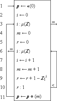 |
Legend |
Program 3.9 Partitioning of the left list of an n-tuply rooted tree
|
Example 3.1. Partitioning of an n-tuply rooted tree.
Program 3.9 shows a scheme
for partitioning a left list Z of a tree T
into component subtrees,
i.e., for determining the vector p
such that pj
is the moment of the singular subtree
Tj.
Thus ν(p) = μ1(T),
pj = μ(Tj),
and the infix
The loop 6-10 scans successive components of the degree vector Z1 (in ascending order) and computes r, the indicated number of roots. The value of r increases by, at most, one per iteration, and when r becomes unity, the end of a singly rooted tree has been reached. Its moment m is then appended (step 11) as a new final component of the partition vector p, the parameters m and r are reset, and the scan of the next rooted tree is begun. Normal termination occurs at step 3; termination at step 6 indicates ill formation of Z. |
 |
Figure 3.10 Construction of a Huffman prefix code
|
Example 3.2. Huffman minimum redundancy prefix code. If b is any set such that ν(b) > 1, then any other finite set a can be encoded in b, that is, represented by b. (The sets a and b may be called the “alphabet” and “basic alphabet”, respectively.) If ν(a) ≤ ν(b), the encoding may be described by a mapping vector k such that ⍴(ai) = bki. If ν(a) > ν(b), then each ai must be represented by a vector xi ⊆ b. For example, if a = ⍳0(10) and b = ⍳0(2), then the decimal digits a may be encoded in the so-called 8421 system:
In so-called fixed length coding the vectors xi have a common dimension d, and the decoding of a message m (consisting of the catenation of vectors xi) involves the selection of successive infixes of dimension d. If the probability distribution of the characters a1 occurring in messages is not uniform, more compact encoding may be achieved by using variable length codes and assigning the shorter codes to the more frequent characters. Decoding of a message in variable length coding can be performed only if the boundaries between the successive xi are indicated in some way. The boundaries between characters in a message in variable length code may be demarked by special partition symbols (which is inefficient) or by using a prefix code in which no legitimate code point xi is the prefix of any other legitimate code point, including itself. The index vectors of the leaves of any tree possess this property; conversely, any set of prefix codes can be arrayed as the leaves of some tree. Hence if each character of the set to be encoded is assigned as the leaf of a common tree, and if each character is encoded by the associated index vector, a so-called prefix code is attained. Figure 3.10 furnishes an example of a binary code (i.e., the branching ratios do not exceed two) constructed in this manner. 0-origin indexing is used. The discussion will be limited to binary trees. If fi
is the frequency of the ith character
and li
is the length of the assigned code
(i.e., the length of path to the root),
then the most efficient code is attained by
minimizing the scalar product
Programs 3.11 and 3.12 show the construction of the tree T representing a Huffman code for a set of characters ci with frequencies fi the former in terms of the tree itself and the latter in terms of its left list. |
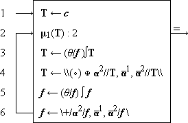
|
Program 3.11 Construction of the binary Huffman code T
for characters c with frequency f
|
Program 3.11. The frequency vector f is permuted (step 5) to bring it to ascending order, and the tree is subjected (step 3) to the same permutation. Step 4 replaces the first two rooted subtrees of T by the single subtree obtained by rooting them in a null, and step 6 makes the corresponding alterations in the frequency vector. The tree is initialized (step 1) as a one-level tree whose roots are the given characters, and the process terminates when the number of roots of T has been reduced to two. |
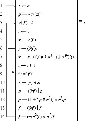 |
Legend Program 3.12 Construction of the left list z |
|
Program 3.12. The tree T of Program 3.11 is represented
by the left list node vector z,
in conjunction with the implicit degree vector
Program 1.21 can be applied to the left list produced by Program 3.12 to determine the associated index matrix (in a 0-origin system), and hence the actual codes assigned. It is not essential that the characters be assigned to leaves in precisely the order specified by Programs 3.11 and 3.12, and it is sufficient that the dimension of the leaf index increase monotonically with decreasing frequency of the character. It is therefore unnecessary to carry the characters themselves through the process; it suffices to determine the structure of the tree, sort the corresponding index matrix to right list order (which is ordered on dimension of the index vectors), and assign the characters (in decreasing order by frequency) to successive leaves. Since the structure of such a tree (whose nodes have a common irrelevant value and whose nonleaves all have a common branching ratio equal to the number of roots) is sufficiently determined by the moment vector μ(T), the process of Program 3.12 can be simplified. |
Chain list matrices
The full chain list matrix of a tree T
is a matrix P of dimension
|
(a) |
(b) |
(c) |
|
|||||||||||||||||||||||||||||||||||||||||||||||||||||||||||||||||||||||||||||||||||||||||||||||||||||||||||||||||||||||||||||||||||||||||||||||||||||||||||||||||||||||||||||||||||||||||||||||||||||||||||||||||||||||||||||||||||||||||||||||||||||||||||||||||||||||||||||||||||||||||||||||||||||||||||||||||||||||||||||||||||||||||||||||||||||||||||||||||||||||||||||||||||||||||||||||||||||||||||||||||||||||||||||||||||||
Table 3.13 Chain lists of the tree of Fig. 1.16
The full chain list matrix is a formalization
of the scheme suggested
in the discussion of chained representations (Sec. 3.2).
Its convenience in forward path tracing is obvious.
Since it does not identify the roots of the tree,
an auxiliary vector must be provided for this purpose.
However, if the ordering chosen for the nodes
is that of a right list,
the roots occur first in the list,
their number
2/P
The right chain list matrix of a tree T
is therefore defined as
3/P,
For a search of the type described by Program 3.14, it is necessary to scan down a level until agreement is reached and then across to the next level. For this type of scan, the filial-heir chain list is compact and convenient.
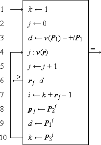 |
Legend |
Program 3.14 Determination of the path p
= Tr
from the right chain list matrix P
The set of (j + 1)th level nodes
of the subtree Ti are collectively called
the jth filial vector of node i,
and the first member of the first filial vector of
node i is called the heir of node i.
(For brevity, the first filial vector of a
node will also be called its filial vector.)
If each node is chained only to its successor
in the filial vector containing it and to its heir,
the resulting representation is called
a filial-heir chain list.
Formally, the filial-heir representation of a tree T
is a matrix F of dimension
References
| • | Blaauw, G. A., (1959), “Indexing and Control-Word Techniques”, IBM Journal of Research and Development, vol. 3, pp. 288-301. |
| • | Brooks, F.P., Jr., and K.E. Iverson, (1962), (in press) Automatic Data Processing, Wiley, New York. |
| • | Burks, A.W., D.W. Warren, and J.B. Wright, (1954), “An Analysis of a Logical Machine Using Parenthesis-free Notation”, Mathematical Tables and Other Aids to Computation, vol. VIII, pp. 53-57. |
| • | Dewey, Godfrey, (1923), Relative Frequency of English Speech Sounds, Cambridge University Press, p. 185. |
| • | Huffman, D.A., (1952), “A Method for the Construction of Minimum Redundancy Codes”, Proc. IRE, vol. 40, pp. 1098-1101. |
| • | Iverson, K.E., (1955), “Report by the Staff of the Computation Laboratory to the American Gas Association and Edison Electric Institute”, Section III, Report No.1, Harvard Computation Laboratory. |
| • | Johnson, L.R., (1962), “On Operand Structure, Representation, Storage, and Search”, Research Report # RC-603, IBM Corp. |
| • | Lukasiewicz, Jan, (1951), Aristotle’s Syllogistic from the Standpoint of Modern Formal Logic, Clarendon Press, Oxford, England, p. 78. |
| • | Marimont, R.B., (1959), “A New Method of Checking the Consistency of Precedence Matrices”, J. ACM, vol. 6, pp. 164-171. |
| • | Ross, I.C., and F. Harary, (1960), “The Square of a Tree”, Bell System Tech. J., vol. XXXIX, pp. 641-8. |
| • | Shaw, J.C., A. Newell, H.A. Simon, and T.O. Ellis, (1958), “A Command Structure for Complex Information Processing”, Proc. Western Joint Computer Conference, pp. 119-128. |
Notes
Exercises
The symbols a and c will be used exclusively to denote lower case and capital alphabets defined as follows:
| a = | (0, a, b, c, … , z, ., ,, #, *, +). | |
| c = | (0, A, B, C, … , Z, ., ,, #, *, +). |
The expression
3.1 For each of the following cases, specify a suitable encoding matrix and format vector and show the explicit value of the infix of π which (in a solid representation) represents the given example vector x:
| (a) | the decimal digits
d = ⍳0(10)
in a ranked fixed-length code
for π ⊆ ⍳0(2). Example: x = (6, 8, 9). |
| (b) | the set a
in a ranked fixed-length code
for π ⊆ ⍳0(2). Example: x = (c, a, t). |
| (c) | the set
a ∪ c ∪ ⍳0(10)
in a fixed-length code
for π ⊆ ⍳0(10). Example: x = (M, a, y, ∘, 3, ,, 1,9,6,0, .). |
| (d) | the set a ∪ c
in a two-case code (with single-character shift)
for π ⊆ a.
(See Brooks and Iverson, 1962.) Example: x = (T, r, o, y, ,, N, ., Y, .). |
| (e) | the set a
in a Huffman prefix code
for π ⊆ ⍳0(2).
Assume the frequency distribution given in
Dewey (1923). Example: x = (t, r, e, e). |
3.2 For each of the cases of Exercise 3.1
write a program which decodes the infix
3.3 The ordered set of months m = (JANUARY, FEBRUARY, … , DECEMBER) is to be represented by the physical vector π ⊆ c ∪ ⍳0(10). For each of the following types of representation, specify a particular representation and show the values of the relevant components of π:
| (a) | a linear representation (employing null elements for filling to a common dimension in π). |
| (b) | a solid representation for each element of m and an appropriate grid matrix itself represented linearly. |
| (c) | a chained representation. |
| (d) | a double chained representation. |
3.4
| (a) | For each of the cases of Exercise 3.3, write a program which selects month mk. |
| (b) | Trace each program for the case k = 2. |
| (c) | For case (d) of Exercise 3.3, write a program which selects mk by forward chaining if k ≤ ν(m)÷2, and by backward chaining if k > ν(m)÷2. |
3.5 For each of the cases of Exercise 3.3,
write a program which “prints out”
the set of months in a minimum number of n-character lines,
inserting a single null between successive months except where
(i) further nulls must be added to prevent the continuation
of a single word from one line to the next, or
(ii) no null is needed between two successive words,
the first of which is coterminous with the line.
In other words, produce a matrix Z
of row dimension n and of minimum
column dimension such that
(Z ≠ ∘E)/Z =
⍴(m1)
⍴(m2) …
⍴(m12),
and such that each row Zi
may be partitioned into one or more vectors of the form
∘∊,
3.6 Assuming a linear representation for each of the logical vectors involved, and a forward-chained representation for each of the remaining operands, write programs for the following operations. Assume in each case that the arguments x and y need not be retained, and assume the use of a backward-chained pool where necessary.
| (a) | z ← \x, u, y\ |
| (b) | z ← /x, u, y/ |
| (c) | z ← k ↑ x |
| (d) | z ← k ↓ x |
3.7 Repeat Exercise 3.6(a), using separate grid matrices for x, y, and z instead of chained representations. Specify a suitable linear representation for each of the grid matrices.
3.8
| (a) | If a chained representation is used for a vector x, then the selection of a specified component can be made faster by providing a number of alternative starting points for the required scan. State precisely the quantities required in such a process and write a program showing its use. |
| (b) | If provision is made for starting the scan at any component of x, the chained representation may itself be simplified. Show precisely what the simplified form is and identify the type of representation to which it is equivalent. |
3.9 Frequently a vector x kept in a partitioned representation (for efficient use of storage) must be “unpacked” to a linear or other more accessible form for efficient processing. The converse operation of “packing” is also required. Let the partitioned representation be a file Φ employing an intercomponent partition λ1, and a terminal partition λ2, and write both packing and unpacking programs for each of the following cases. Assume that the maximum dimension in π of any component is n.
| (a) | A solid linear representation employing null fill. |
| (b) | An allocation prescribed by a grid matrix G with G2 = n∊. |
3.10 Let π ⊆ ⍳0(2),
let the set a be encoded in a five-bit code such that
3.11 For each of the following pool organizations, write a program to convert a given marked pool into a backward-chained pool:
| (a) | dimension-ordered. |
| (b) | address-ordered. |
3.12 For each of the following queue disciplines, write programs which take from and return to the pool an infix of length n. Use secondary linking and relegate to a marked pool any infix which is too short for linking. In each case choose the type of chaining best suited to the particular queue discipline.
| (a) | LIFO (last-in-first-out). |
| (b) | FIFO (first-in-first-out). |
| (c) | Dimension ordered. |
| (d) | Address-ordered (utilize the possibility of fusing adjacent infixes). |
3.13 Give a complete specification of a scheme for representing a tree T by a full chain list matrix which is not in right list order. Write a program (expressed in terms of the physical vector π) which determines the path vector Ti for a given index vector i.
3.14 Give a complete specification of a scheme allowing joint representation of those components shared by two or more of a family of vectors x1, x2, …, xn as suggested in Sec. 3.2. Write programs to (i) select component xji, and (ii) delete component xji.
3.15 Let π ⊆
a ∪ ⍳0(10),
and let
x1, x2, …,
xn
be a family of vectors whose
components belong to the set
1/[a ∪ ⍳0(10)].
3.16 Write a program
which uses the minimization operation
3.17 Let
| (a) | Write a program which determines (as a function of U and r) a suitable row-chained and column-chained representation of X. |
| (b) |
Write a program defined on the representation produced in part (a) to
compute the product
X, |
| (c) | Write a program to determine the trace (that is, +/I/X) of X from the representation produced in part (a). |
3.18 The unique assignment of Huffman codes produced by Program 3.12 is, in general, only one of many equally efficient assignments, since the symbols to be coded need only be assigned, in decreasing order on frequency, to the leaves of the code tree in increasing order on their levels. Show that the structure of the tree produced can be sufficiently described by its moment vector alone, and write a program for the construction of a Huffman code based on this fact.
3.19 Following the notation and terminology used in Program 3.9 for the analogous case of a left list, write a program which determines from the right list R of a tree T, the partition vector p which partitions it by levels.
3.20 Write a program which determines the right list R = ⍺2/]T as a function of the left list L = ⍺2/[T. Incorporate tests of well formation.
3.21 Let [X]p
denote the pth power
of the square matrix X
with respect to the operators
1 and
2,
that is,
[X]p =
X
X …
X
to p factors.
| (a) |
Show that
([C ]p)ji = 1
if and only if there is a path of length p from
node i to node j in the graph (n, C). ]p)ji = 1
if and only if there is a path of length p from
node i to node j in the graph (n, C).
|
| (b) |
Show that [C]p = 0
for some p < ν(C)
if and only if (n, C)
contains no circuits.
|
| (c) | If (n, C) contains no circuits, the connection matrix C is said to be “consistent”. The result of part (a) can be used to check consistency. Program the alternative method of Marimont (1959). |
| (d) |
If H = C ∨ I, then
([H]p)ji = 1
if and only if i = j
or there exists a path
from node i to node j
of length ]p |
3.22 Devise programs to determine
| (a) | whether a given connection matrix C represents a tree. | ||||
| (b) | the left list of the tree (n, C). | ||||
| (c) | the right list of the tree (n, C). | ||||
| (d) |
a node list n and connection matrix C as a function of
|
3.23 Show that (n, C) and (np, Cpp) represent the same graph for any permutation p.
3.24 If (n, C)
is a tree and if C,
Summary of Notation
S.1 Conventions
Basic conventions
| (a) | 1-origin indexing assumed in this summary. | |
| (b) | Controlling variables appear to the left, e.g., u/x, u ⊥ y, k ↑ x, and u ⌈ x. | |
| (c) | Dimension n may be elided (if determined by compatibility) from ∊(n), ∊k(n), ⍺k(n), ⍵k(n), and ⍳ j(n). | |
| (d) | The parameter j may be elided from operators | j, θ j, ∫ j, and ⍳ j, and from the vector ⍳ j if j is the index origin in use. | |
| (e) | The parameter k may be elided from k ↑ x if k = 1. |
Branching conventions
| (a) |
│ x : y │ The statement to which the arrow leads is executed
if | |
| (b) |
x : y, r → s The statement numbered s i
is executed next if (xr i y) = 1.
The null symbol ∘ occurring as a component
of r denotes the relation
which complements the disjunction
of the remaining relations in r.
| |
| (c) |
→ Program a, b Program a branches to its statement b. The symbol a may be elided if the statement occurs in Program a itself. |

Operand conventions used in summary
| Scalar | Vector | Matrix | Tree | |||||
| Logical | u, v, w | u, v, w | U, V, W | U, V, W | ||||
| Integral | h, i, j, k | h, i, j, k | H, I, J, K | H, I, J, K | ||||
| Numerical | x, y, z | x, y, z | X, Y, Z | X, Y, Z | ||||
| Arbitrary | a, b, c | A, B, C | A, B, C | A, B, C |
S.2 Structural Parameters, Null
| Dimension | ν(a) | Number of components in vector a |  |
|||||||||||
| Row dimension | ν(A) | Number of components in each row vector Ai |
|
|||||||||||
| Column dimension | μ(A) | Number of components in each column vector Aj |
|
|||||||||||
| Height | ν(A) | Length of longest path in A | |
|||||||||||
| Moment | μ(A) | Number of nodes in A | |
|||||||||||
| Dispersion vector | ν(A) |
|
|
|||||||||||
| Moment vector | μ(A) | μ j(A) = number of nodes on level j
of A; |
|
|||||||||||
| Degree of node i | δ(i, A) | Degree of node i of tree A | |
|||||||||||
| Degree | δ(A) | δ(A) = max δ(i, A) i |
|
|||||||||||
| Leaf count | λ(A) | λ(A) is the number of leaves in A | |
|||||||||||
| Row dimension of file | ν(Φ) | Number of files in each row of a file array |
|
|||||||||||
| Column dimension of file | μ(Φ) | Number of files in each column of a file array |
|
|||||||||||
| Null character | ∘ | Null character of a set (e.g. space in the alphabet) or null reduction operator | |
S.3 Relations
| Equality | a = b | a and b are identical | | |||
| Membership | a ε b | a = bi for some i | | |||
| Inclusion | b ⊇ a
a ⊆ b |
aj = b for all j | | |||
| Strict inclusion | b ⊃ a
a ⊂ b |
b ⊇ a and a  b b |
| |||
| Similarity | b ≡ a | b ⊇ a and a ⊇ b | | |||
| Complementary relations |  |
The relation which holds if and only if R does not.
Examples of complementary pairs:
; ; ; . . | ||||
| Combined (ored) relations | A list of relations between two variables
is construed as the or of the relations.
Thus |
S.4 Elementary Operations
| Negation | w ← |
w = 1 ←→ u = 0 | | ||
| And | w ← u ∧ v | w = 1 ←→ u = 1 and v = 1 | | ||
| Or | w ← u ∨ v | w = 1 ←→ u = 1 or v = 1 | | ||
| Relational statement | w ← |
w = 1 ←→
the relation |
| ||
| Sum | z ← x + y | z is the algebraic sum of x and y | | ||
| Difference | z ← x – y | z is the algebraic difference of x and y | | ||
| Product |
z ← x × y z ← xy c ← a × u c ← au |
z is the algebraic product of numbers x and y, and c is the arbitrary character a or zero according to whether the logical variable u is one or zero. | | ||
| Quotient | z ← x ÷ y | z is the quotient of x and y | | ||
| Absolute value | z ← |x| | z = x × [(x > 0) – (x < 0)] | | ||
| Floor | k ← ⌊x⌋ | k ≤ x < k + 1 | | ||
| Ceiling | k ← ⌈x⌉ | k ≥ x > k – 1 | | ||
| j-Residue mod h | k ← h| j i | i = hq + k; j ≤ k < j + h; and q is integral. | |
S.5 Vector Operations
| Component-by-component extension of basic operation | c ← a b | ci ← ai bi .
Examples:
x × y,
(a ≠ b),
h| j i,
u ∧ ,
⌈x⌉. |
| ||||
| Scalar multiple |
z ← x × y z ← xy c ← a × u c ← au | z i ← x × yi, and ci ← a × ui | | ||||
| Reduction | c ← /a | c = (…((a1 a2)
a3)…) aν),
| | ||||
|
where is a binary operator
or relation with a suitable domain. Examples:
+/x,
×/x,
≠/u.
Reduction of the null vector ∊(0)
is defined as the identity element
of the operator .
Examples:
+/∊(0) = 0,
×/∊(0) = 1,
∨/∊(0) = 0,
∧/∊(0) = 1. | |||||||
| Ranking | | ||||||
| j-origin b-index of a | c ← b ⍳j a | c = ∘ if a b;
otherwise c is the j-origin index
of the first occurrence of a in b. | |||||
| j-origin b-index of a | c ← b ⍳j a | ci = b ⍳j ai | |||||
| Left rotation | c ← k ↑ a | ci = a j, where j = ν(a) |1 (i + k) | | ||||
| Right rotation | c ← k ↓ a | ci = a j, where j = ν(a) |1 (i – k) | | ||||
| Base y value of x | z ← y ⊥ x | z = +/(p × x),
where pν = 1, and
pi–1 = pi × yi | | ||||
| Compression | c ← u/b | c is obtained from b by suppressing each bi for which ui = 0 | | ||||
| Expansion | c ← u\b | /c = 0,
u/c = b |
| ||||
| Mask | c ← /a,u,b/ | /c = /a,
u/c = u/b |
| ||||
| Mesh | c ← \a,u,b\ | /c = a,
u/c = b |
| ||||
| Catenation | c ← a b | c = (a1, a2,… aν(a),
b1, b2,… bν(b)) = \a, ⍵ν(b), b\ |
| ||||
| Characteristic of x on y | w ← ∊yx | wi = (yi ε x); ν(w) = ν(y) | | ||||
| jth unit vector | w ← ∊ j(h) | wi = (i = j) |  |
| |||
| Full vector | w ← ∊(h) | wi = 1 | | ||||
| Zero vector | w ← (h) w ← 0 | wi = 0 | ν(w)=h | | |||
| Prefix of weight j | w ← ⍺ j(h) | First k of wi are unity, where k = min( j,h). |
| ||||
| Suffix of weight j | w ← ⍵ j(h) | Last k of wi are unity, where k = min( j,h). |
| ||||
| Maximum prefix | w ← ⍺/u | w is the max length prefix in u. | | ||||
| e.g. ⍺/(1, 1, 0, 1, 0, 1) = (1, 1, 0, 0, 0, 0). | |||||||
| Maximum suffix | w ← ⍵/u | w is the max length suffix in u. | | ||||
| e.g. ⍵/(1, 1, 0, 1, 0, 1) = (0, 0, 0, 0, 0, 1). | |||||||
| Forward set selector | w ← σ/a | wi = 1 if a j ≠ a i for all j < i | | ||||
| Backward set selector | w ← τ/a | wi = 1 if a j ≠ a i for all j > i | | ||||
| Maximum selector | w ← u⌈x | wi = ui
∧ (xi = m) where
m = max(u/x)j j |
| ||||
| Minimum selector | w ← u⌊x | wi = ui
∧ (xi = m) where
m = min(u/x)j j |
| ||||
| Interval or j-origin identity permutation vector | k ← ⍳j(h) | k = (j, j+1, …, j+h–1) | | ||||
| j-origin identity permutation vector | k | k = ⍳j(ν(k)) | | ||||
| j-origin mapping | c ← ab c ← b∫ja | ci = ∘
if bi
⍳j(ν(a));
otherwise ci =
abi
in a j-origin system for a.
In the first form (that is, c ← ab),
the origin cannot be specified directly. |
| ||||
| j-origin ordering | k ← θj/x | y = k ∫j x is in ascending order and original relative ordering is maintained among equal components, that is, either yi < yi+1 or yi = yi+1 and ki < ki+1 | | ||||
S.6a Row Generalizations of Vector Operations
| Z ← X
Y |
Z j i =
X j i
Y j i |
|
|||
| z ← /X
|
z i =
/X i |
|
|||
| C ← /A
|
C = A1
A2
…
Aν |
|
|||
| M ← B ⍳h A | M i = B i ⍳h A i | |
|||
| C ← k ↑ A | C i = k i ↑ A i | |
|||
| C ← k ↓ A | C i = k i ↓ A i | |
|||
| z ← Y ⊥ X | z i = Y i ⊥ X i | |
|||
| C ← Ab | C j = Abj | |
|||
| C ← B ∫h A | C i = B i ∫h A i | |
|||
| K ← θh/X | K i = θh/X i | |
|||
| C ← A
B |
C i = A i
B i |
|
|||
| C ← u/B | C i = u/B i | |
|||
| c ← U/B | c = U1/B1
…
U μ/B μ |
|
|||
| C ← u\B | /C = 0, |
u/C = B | |
||
| C ← U\b |  /C = 0, /C = 0, |
U/C = b | |
||
| C ← \A, u, B\ | /C = A, |
u/C = B | |
||
| C ← \a, U, b\ | /C = a, |
U/C = b | |
||
| C ← /A, u, B/ | /C = /A, |
u/C = u/B | |
||
| C ← /A, U, B/ | /C = /A, |
U/C = U/B | |
||
| C ← /a, U, b/ | C = /E\a, U, E\b/ | |
|||
| W ← ⍺/U | W i = ⍺/U i | |
|||
| W ← ⍵/U | W i = ⍵/U i | |
|||
| W ← σ/U | W i = σ/U i | |
|||
| W ← τ/U | W i = τ/U i | |
|||
| W ← U⌈X | W i = U i⌈X i | |
|||
| W ← U⌊X | W i = U i⌊X i | |
|||
S.6b Column Generalizations of Vector Operations
| Z ← X
Y |
Z j i =
X j i
Y j i |
|
|||
| z ← //X
|
z j =
/X j |
|
|||
| C ← //A
|
C = A1
A2
…
Aμ |
|
|||
| M ← B ⍳⍳h A | M j = B j ⍳h A j | |
|||
| C ← k
A |
C j = k j ↑ A j | |
|||
C ← k  A
A |
C j = k j ↓ A j | |
|||
| z ← Y
X |
z j = Y j ⊥ X j | |
|||
| C ← Ab | C i = Abi | |
|||
| C ← B ∫∫h A | C j = B j ∫h A j | |
|||
| K ← θh//X | K j = θh/X j | |
|||
| C ← A
B |
C j = A j
B j |
||||
| C ← u//B | C j = u/B j | |
|||
| c ← U//B | c = U1/B1
…
U ν/B ν |
|
|||
| C ← u\\B | //C = 0, |
u//C = B | |
||
| C ← U\\b | //C = 0, |
U//C = b | |
||
| C ← \\A, u, B\\ | //C = A, |
u//C = B | |
||
| C ← \\a, U, b\\ | //C = a, |
U//C = b | |
||
| C ← //A, u, B// | //C = //A, |
u//C = u//B | |
||
| C ← //A, U, B// | //C = //A, |
U//C = U//B | |
||
| C ← //a, U, b// | C = /E\\a, U, E\\b/ | |
|||
| W ← ⍺//U | W j = ⍺/U j | |
|||
| W ← ⍵//U | W j = ⍵/U j | |
|||
| W ← σ//U | W j = σ/U j | |
|||
| W ← τ//U | W j = τ/U j | |
|||
| W ← U⌈⌈X | W j = U j⌈X j | |
|||
| W ← U⌊⌊X | W j = U j⌊X j | |
|||
S.7 Special Matrices
| Full matrix | W ← E(p, q) | Wji = 1 |  |
μ(W) = p ν(W) = q, for p and q integers. Elision of p and q if dimensions determined by compatibility. |
| |||
| Zero matrix | W ← (p, q) | Wji = 0 | | |||||
| W ← 0 | ||||||||
| Superdiagonal | W ← kI(p, q) | Wji = (i + k = j) | | |||||
| Identity | W ← I(p, q) | W = 0I(p, q) | | |||||
| Upper left (triangle) | W ← (p, q) | Wji |  |
= (i + j ≤ m), m = min(p, q) |
| |||
| Upper right | W ← (p, q) |  |
| |||||
| Lower left | W ← (p, q) |  |
| |||||
| Lower right | W ← (p, q) |  |
| |||||
S.8 Transposition
| Diagonal |
C ← |
Ci j = |  Bj i Bj i |
| ||
|
C ← |
| |||||
| Counter diagonal |
C ← |
 |
| |||
| Horizontal |
C ← |
 |
| |||
| Vertical |
C ← |
 |
| |||
| Vector |
y ← y ← |
y ← xν + 1 – i | |
S.9 Set Operations
| Intersection | c ← b ∩ a | c = ∊ba/b | |
|||
| Difference | c ← b ∆ a | c = ba/b |
|
|||
| Union | c ← b ∪ a | c = b (a ∆ b) |
|
|||
| Cartesian product | C ← b1
… bn | C 1 + d ⊥ (k – ∊)
= (bk11,
bk22, …,
bknn);
d j = ν(b j);
1 ≤ k j ≤ d j Clearly, ν(C) = n, and μ(C) = ×/d |
|
S.10 Generalized Matrix Product
| C ← A
B |
C j i =
1/(A i
2 B j),
where 2 produces a vector
(i.e., is not the operator ⊥), and
1
is a reduction operator (and hence
C j i
is a scalar). |
|
||
| C ← A
b |
C i =
(A i
b),
where is any operator
which produces a vector of dimension ν(b).
|
|
||
| C ← a
B |
C j =
(a
B j),
where is any operator
which produces a vector of dimension ν(a). |
|
||
| C ← a
b |
C j i =
(a i
b j). |
|
S.11 Files
| File | Φ j i | A representation of a of the form (p1, a1, p2, a2, …, aν(a), pν(a)+1, ∘, pν(a)+2, …, pν(p)), where ph is the partition at position h, |
|
||
| Position file | π(Φ j i) ← h | Set file to position h. Called rewind if h = 1, and wind if h = ν(p). | |
||
| Record (from position h) | |||||
| Forward | 0Φ j i ← a, λk | ah ← a,
ph+1 ← λk;
stop at position |
|
||
| Backward | 1Φ j i ← a, λk | ah–1 ← a,
ph–1 ← λk;
stop at position |
|
||
| Read (from position h) | |||||
| Forward | a, b ← 0Φ j i | a ← ah;
b ← ph+1;
stop at position |
|
||
| Backward | a, b ← 1Φ j i | a ← ah–1;
b ← ph–1;
stop at position |
|
||
| File array | |||||
| Full | Φ | Array of files Φ j i,
for |
|
||
| Row | Φ i | Row of files Φ j i,
for |
|
||
| Column | Φ j | Column of files Φ j i,
for |
|
||
| Compression | |||||
| Row | u/Φ | Selection as in corresponding operations on matrices. | |
||
| Column | u//Φ | ||||
S.12 Trees
| Path i | c ← Ai | c1 is the i1th root of A; c j is the i j th node of the nodes on level j reachable from node c j–1. | |
||
| Node i | c ← (Ai)ν(i) | The final node of path Ai. | |
||
| Subtree i | C ← A i | C is the subtree of A rooted in node i. | |
||
| Component-by- component |
C ← A B |
(C i)ν(i)
=
(A i)ν(i)
(B i)ν(i). |
|
||
| Path reduction | C ← /A |
Reduction by operator or relation
on nodes in left list order. |
|
||
| Level reduction | C ← //A |
Reduction by operator or relation
on nodes in right list order. |
|
||
| j-origin b-index | B ← b ⍳j A | (B i)ν(i) = b ⍳j ((Ai)ν(i)) | |
||
| j-origin mapping | C ← b ∫j A | Rooted subtree Ci is a single null character node if bi ∉ ⍺j(μ1(A)); otherwise Ci = Abi, where A is treated in a j-origin system. | |
||
| Full right list matrix |
C ← ]A | |
The rows of the index matrix
2/C
are the right (left) justified index vectors
(with null fill to the common dimension ν(A))
arranged in increasing order;
C1 and C2
are the corresponding degree and node vectors of A. |
|
|
| Full left list matrix |
C ← [A | ||||
| Right list matrix | C ← ⍺2/]A | |
The degree and node vector columns of the full right (left) list. | |
|
| Left list matrix | C ← ⍺2/[A | ||||
| Tree compression | C ← U/A | C is obtained from A by suppressing node i if node i of U is zero and reconnecting so that for each remaining pair of nodes, the one lies in the subtree rooted at the second if and only if it did so in A. | |
||
| Path compression | C ← u/A | C is obtained from A by suppressing all nodes
on level j if |
|
||
| Level compression | C ← u//A | C is obtained from A by suppressing rooted subtree Aj if uj = 0. | |
||
| Level mesh | C ← \\A, u, B\\ | //C = A; u//C = B. |
|||
| Level mask | C ← //A, u, B// | //C = //A;
u//C = u//B. |
|||
| Path catenation | C ← A B |
C is obtained by connecting roots of B to leaves of A, allotting successive groups of at most ⌈μ1(B) ÷ λ(A)⌉ roots of B to each successive leaf of A. | |
||
| Full tree | W ← E | Each node of W is unity and the structure of W is determined by compatibility. | |
||
| W ← E(k) | Each node of W is unity; W is homogeneous (i.e., all nodes on any level have a common degree) and ν(W) = k. | |
|||
| Zero tree | W ←  W ← 0 |
 |
Each node of W is zero and the structure of W is determined by compatibility. | |
|
| W ← (k) |
Each node of W is zero; W is homogeneous and ν(W) = k. | |
|||
| Path tree | W ← uE | /W = 0;
u/W = E;
structure of W determined by compatibility. |
|
||
| W ← uE(k) | /W = 0;
u/W = E;
W is homogeneous and ν(W) = k. |
|
|||
| Level tree | W ← uE | //W = 0;
u//W = E;
structure of W determined by compatibility. |
|
||
| W ← uE(k) | //W = 0;
u//W = E;
W is homogeneous and ν(W) = k. |
|
|||
| Maximization | W ← U ⌈ A | |
W = U ∧ (A = mE), where m is the maximum (minimum) over all nodes of U/A. | |
|
| Minimization | W ← U ⌊ A | ||||
| Maximum path prefix | W ← ⍺/U | W is obtained from U by zeroing all nodes of every subtree rooted in a zero node. | |
||
| Maximum path suffix | W ← ⍵/U | W is obtained from U by zeroing every node which contains a zero node in its subtree. | |
||
| Forward path set selector | W ← σ/A | (W i)ν(i) = 1 if (Ai)ν(i) differs from all preceding nodes of path Ai. | |
||
| Backward path set selector | W ← τ/A | (W i)ν(i) = 1 if (Ai)ν(i) differs from all other nodes in its subtree. | |
||
| Maximum level prefix | W ← ⍺//U | ∊ j/W = ⍺/∊ j/U | |
||
| Maximum level suffix | W ← ⍵//U | ∊ j/W = ⍵/∊ j/U | |
||
| Forward level set selector |
W ← σ//A | ∊ j/W = σ/∊ j/U | |
||
| Backward level set selector | W ← τ//A | ∊ j/W = τ/∊ j/U | |
Originally appeared as A Programming Language, Wiley, 1962, available as a pdf file from here.
| created: | 2009-10-13 21:35 |
| updated: | 2019-10-17 15:15 |