Programming Style in APL
Kenneth E. Iverson
IBM Thomas J. Watson Research Center
Yorktown Heights, New York
When all the techniques of program management and programming practice have been applied, there remain vast differences in quality of code produced by different programmers. These differences turn not so much upon the use of specific tricks or techniques as upon a general manner of expression, which, by analogy with natural language, we will refer to as style. This paper addresses the question of developing good programming style in APL.
Because it does not rest upon specific techniques, good style cannot be taught in a direct manner, but it can be fostered by the acquisition of certain habits of thought. The following sections should therefore be read more as examples of general habits to be identified and fostered, than as specific prescriptions of good technique.
In programming, as in the use of natural languages, questions of style depend upon the purpose of the writing. In the present paper, emphasis is placed upon clarity of expression rather than upon efficiency in space and time in execution. However, clarity is often a major contributor to efficiency, either directly, in providing a fuller understanding of the problem and leading to the choice of a better, more flexible, and more easily documented solution, or indirectly, by providing a clear and complete model which may then be adapted (perhaps by programmers other than the original designer) to the characteristics of any particular implementation of APL.
All examples are expressed in 0-origin.
Examples chosen from fields unfamiliar
to any reader should perhaps be skimmed
lightly on first reading.
1. Assimilation of Primitives and Phrases
Knowledge of the bare definition of a primitive can permit its use in situations where its applicability is clearly recognizable. Effective use, however, must rest upon a more intimate knowledge, a feeling of familiarity, an ability to view it from different vantage points, and an ability to recognize similar uses in seemingly dissimilar applications.
One technique for developing intimate knowledge of a primitive or a phrase is to create at least one clear and general example of its use, an example which can be retained as a graphic picture of its behavior when attempting to apply it in complex situations. We will now give examples of creating such pictures for three important cases, the outer product, the inner product, and the dyadic transpose.
Outer product. The formal definition of the result of the expression r←a∘.f b for a specified primitive f and arrays a and b of ranks 3 and 4 respectively, may be expressed as:
r[h;i;j;k;l;m;n] ←→ a[h;i;j] f b[k;l;m;n]
Although this definition is essentially complete, it may not be very helpful to the beginner in forming a manageable picture of the outer product.
To this end it might be better to begin with the examples:
     n∘.+n←1 2 3 4                  n∘.×n
2 3 4 5                         1  2  3  4
3 4 5 6                         2  4  6  8
4 5 6 7                         3  6  9 12
5 6 7 8                         4  8 12 16
and emphasize the fact that these outer products are the familiar addition and multiplication tables, and that, more generally, a∘.f b yields a function table for the function f applied to the sets of arguments a and b .
One might reinforce the idea by examples in which
the outer product illuminates the definition, properties,
or applicability of the functions involved.
For example, the
expressions
Useful pictures of outer products of higher rank may also be formed. For example, d∘.∨d∘.d←0 1 gives a rank three function table for the or function with three arguments, and if a is a matrix of altitudes of points in a rectangular area of land and c is a vector of contour levels to be indicated on a map of the area, then the expression c∘.≤a relates the points to the contour levels and +⌿c∘.≤a gives the index of the contour level appropriate to each point.
Inner Product. Although the inner product is perhaps most used with at least one argument of rank two or more, a picture of its behavior and wide applicability is perhaps best obtained (in the manner employed in Chapter 13 of Reference 1) by first exploring its significance when applied to vector arguments. For example:
| p←2 3 5 7 11 | |
| q←2 0 2 1 0 | |
| +/p×q 21 |
Total cost in terms of price and quantity. |
| ⌊/p+q 3 |
Minimum trip of two legs with distances to and from connecting point given by p and q . |
| ×/p*q 700 |
The number whose prime factorization is specified by the exponents q . |
| +/p×q 21 |
Torque due to weights q placed at positions q relative to the axis. |
The first and last examples above illustrate the fact that the same expression may be given different interpretations in different fields of application.
The inner product is defined in terms of expressions of the form used above.
Thus, p+.×q ←→ +/p×q and,
more generally for any pair of scalar
functions f and g ,
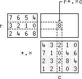
The +.× inner product applied to two vectors v and w (as in v+.×w) can be construed as a weighted sum of the vector v , whose elements are each “weighted” by multiplication by the corresponding elements of w , and then summed. This notion can be extended to give a useful interpretation of the expression m+.×w for a matrix m , as a weighted sum of the column vectors of m . Thus:
      w←3 1 4
      ⎕←m←1+3 3⍴⍳9
1 2 3
4 5 6
7 8 9
      m+.×w
17 41 65
This result can be seen to be equivalent to writing the elements of w below the columns of m , multiplying each column vector of m by the element below it, and adding.
If w is replaced by a boolean vector b (whose elements are zeros or ones), then m+.×b can still be construed as a weighted sum, but can also be construed as sums over subsets of the rows of m , the subsets being chosen by the 1’s in the boolean vector. For example:
      b←1 0 1
      m+.×b
4 10 6
      b/m
1 3
4 6
7 9
      +/b/m
4 10 16
Finally, by using an expression of the form m×.*b instead of m+.×b , a boolean vector can be used to apply multiplication over a specified subset of each of the rows of m . Thus:
      m×.*b
3 24 63
      ×/b/m
3 24 63
This use of boolean vectors to apply functions over specified subsets of arrays will be pursued further in the section on generalization, using boolean matrices as well as vectors.
Dyadic transpose. Although the transposition of a matrix is easy to picture (as an interchange of rows and columns), the dyadic transpose of an array of higher rank is not, as may be seen by trying to compare the following arrays:
      a              1 0 2⍉a               2 1 0⍉a
abcd           abcd                  am
efgh           mnop                  eq
ijkl                                 iu
               efgh
mnop           qrst                  bn
qrst                                 fr
uvwx           ijkl                  jv
               uvwx
                                     co
                                     gs
                                     kw

                                     dp
                                     ht
                                     lx
The difficulty increases when we permit left arguments with repealed elements which produce “diagonal sections” of the original array. This general transpose is, however, a very useful function and worth considerable effort to assimilate. The following example of its use may help.
The associativity of a function f is normally expressed by the identity:
x f (y f z) ←→ (x f y) f z
and a test of the associativity
of the function on some specified
domain
      ⎕←l←d∘.-(d∘.-d)       ⎕←r←(d∘.-d)∘.-d)        l=r
 1 2 3                ¯1 ¯2 ¯3                0 0 0
 0 1 2                ¯2 ¯3 ¯4                0 0 0
¯1 0 1                ¯3 ¯4 ¯5                0 0 0

 2 3 4                 0 ¯1 ¯2                0 0 0
 1 2 3                ¯1 ¯2 ¯3                0 0 0
 0 1 2                ¯2 ¯3 ¯4                0 0 0

 3 4 5                 1  0 ¯1                0 0 0
 2 3 4                 0 ¯1 ¯2                0 0 0
 1 2 3                ¯1 ¯2 ¯3                0 0 0

      ^/,l=r
0

      ⎕←l←d∘.+(d∘.+d)       ⎕←r←(d∘.+d)∘.+d)        l=r
3 4 5                 3 4 5                   1 1 1
4 5 6                 4 5 6                   1 1 1
5 6 7                 5 6 7                   1 1 1

4 5 6                 4 5 6                   1 1 1
5 6 7                 5 6 7                   1 1 1
6 7 8                 6 7 8                   1 1 1

5 6 7                 5 6 7                   1 1 1
6 7 8                 6 7 8                   1 1 1
7 8 9                 7 8 9                   1 1 1
For the case of logical functions, the test made by comparing the function tables can be made complete, since the functions are defined on a finite domain d←0 1 . For example:
      d←0 1
      ∧/,(d∘.∨(d∘.∨d))=((d∘.∨d)∘.∨d)
1
      ∧/,(d∘.≠(d∘.≠d))=((d∘.≠d)∘.≠d)
1
      ∧/,(d∘.⍲(d∘.⍲d))=((d∘.⍲d)∘.⍲d)
0
Turning to the identity for the distribution of one function over another we have expressions such as:
| x×(y+z) ←→ (x×y)+(x×z) |
| and |
| x∧(y∨z) ←→ (x∧y)∨(x∧z) |
Attempting to write the function table comparison for the latter case as:
      l←d∘.∧(d∘.∨d)
      r←(d∘.∧d)∘.∨(d∘.∧d)
we encounter a difficulty since the two sides l and r do not even agree in rank, being of ranks 3 and 4.
The difficulty clearly arises
from the fact that the axes of the left and right function tables
must agree according lo the names in the original identity;
in particular, the x in position 0 on the left
and in positions 0 and 2 on the right implies
that axes 0 and 2 on the right must be “run together”
to form a single axis in position 0.
The complete disposition of the four axes
on the right can be seen to be described
by the vector
      ^/,(d∘.^(d∘.∨d))=0 1 0 2⍉((d∘.^d)∘.∨(d∘.^d))
1
The idea of thorough assimilation discussed thus far in terms of primitive expressions can be applied equally to commonly used phrases and defined functions. For example:
| ⍳⍴v | The indices of vector v | |
| ⍳⍴⍴a | The axes of a | |
| ×/⍴a | The number of elements in a | |
| v[⍋v] | Sorting the vector v | |
| m[⍋+⌿r<.-⍉r←m,0;] | Sorting the rows of m into lexical order | |
| ⍉f⍉m | Applying to columns a function f defined on rows |
Collections of commonly used phrases and functions may
be found in Perlis and Rugaber
[2]
and in Macklin
[3].
2. Function Definition
A complex system should best be designed not as a single monolithic function, but as a structure built from component functions which are meaningful in themselves and which may in turn be realized from simpler components. In order lo interact with other elements of a system, and therefore serve as a “building block”, a component must possess inputs and outputs. A defined function with an explicit argument, or arguments, and an explicit result provides such a component.
If a component function produces side effects by setting global variables used by other components, the interaction between components becomes much more difficult to analyze and comprehend than if communication between components is limited to their explicit arguments and explicit results. Ideally, systems should be designed with communication so constrained and, in practice, the number of global variables employed should be severely limited.
Because the fundamental definition form in APL (produced by the use of ∇ or by ⎕fx , and commonly called the del form) is necessarily general, it permits the definition of functions which produce side effects, which have no explicit arguments, and which have no explicit results. The direct form which uses the symbols ⍺ and ⍵ (as defined in Iverson [4]) exercises a discipline more appropriate to good design, allowing only the definition of functions with explicit results, and localizing all names which are specified within the function, thereby eliminating side effects outside of it.
The direct form of definition may be either simple or conditional. The latter form will be discussed in section 6. The simple form may be illustrated as follows. The expression
f:⍵+4÷⍺
may be read as “f is defined by the expression ⍵+4÷⍺ , where ⍺ represents the first argument of f and ⍵ represents the second”. Thus 8 f 3 yields 3.5 .
If a direct definition is to produce a machine executable function, the definition must be translated by a suitable function. For example, if this translation is called def , then:
      def                          def
f:⍺+÷⍵                       sort:⍵[⍋⍵]
f                            sort
      3 f 4                        sort 3 1 4 3 6 2 7 6
3.25                         1 2 3 3 4 6 6 7

      def                          def
p:+/⍺×⍵*⍳⍴⍺                  pol:(⍵∘.*⍳⍴⍺)+.×⍺
p                            pol
      1 3 3 1 p 4                  1 3 3 1 pol 0 1 2 3 4
125                          1 8 27 64 125
The direct form of definition will be used in the examples which follow.
The question of the translation function def
is discussed in Appendix A.
3. Generality
It is often possible to take a function defined for a specific purpose and modify it so that it applies to a wider class of problems. For example, the function av:(+/⍵)÷⍴⍵ may be applied to a numeric vector to produce its average. However, it fails lo apply to average all rows in a matrix; the simple modification av2:(+/⍵)÷¯1↑⍴⍵ not only permits this, but applies to average the vectors along the last axis of any array, including the case of a vector.
The problem might also be generalized to a weighted average, in which a vector left argument specifies the weights to be applied in summation, the result being normalized by division by the total weight. Again this function could be defined to apply to a vector right argument in the form wav:(+/⍺×⍵)÷+/⍺ , but, applying the inner product in the manner discussed in the preceding section, we may define a function which applies to matrices:
wav2:(⍵+.×⍺)÷+/⍺
Thus:
      ⎕←m←3 4⍴⍳12
0 1  2  3
4 5  6  7
8 9 10 11
      w←2 1 3 4
      w wav2 m
1.9 5.9 9.9
The same function may be interpreted in different ways in different disciplines. For example, if column i of m gives the coordinates of a mass of weight w[i] , then w wav2 m is the center of gravity of the set of masses. Moreover, if the elements of w are required to be non-negative, then the result w wav2 m is always a point in the convex space defined by the points of m , that is a point within the body whose vertices are given by m . This can be more easily seen in the following equivalent function:
wav3:⍵+.×(⍵÷+/⍺)
in which the weights are normalized to sum to 1.
Striving to write functions in a general way not only leads to functions with wider applicability, but often provides greater insight into the problem. We will attempt lo illustrate this in three areas, functions on subsets, indexing, and polynomials.
Functions on subsets. It is often necessary
to apply some function (such as addition or maximum)
over all elements in some subset of a given list.
For example, to sum all non-negative elements in the
list
      x
3 ¯4 2 0 ¯3 7
      x≥0                (x≥0)/x           +/(x≥0)/x
1 0 1 1 0 1        3 2 0 7           12
In general, if b is a boolean vector which defines a subset, we may write +/b/x . However, as seen in the discussion of inner product, this may also be written in the form x+.×b , and in this form it applies more generally to a boolean matrix (or higher rank array) in which the columns (or vectors along the leading axis) determine the different subsets. For example, if
      ⎕←b←(4⍴2)⊤⍳2*4
0 0 0 0 0 0 0 0 1 1 1 1 1 1 1 1
0 0 0 0 1 1 1 1 0 0 0 0 1 1 1 1
0 0 1 1 0 0 1 1 0 0 1 1 0 0 1 1
0 1 0 1 0 1 0 1 0 1 0 1 0 1 0 1
then the columns of b represent all possible subsets
of a vector of four elements,
and if
      x+.×b
0 7 5 12 3 10 8 15 2 9 7 14 5 12 10 17
yields the sums over all subsets of x ,
including the empty set
It is also easy to establish that
      x×.*b
1 7 5 35 3 21 15 105 2 14 10 70 6 42 30 210
yields the products over all subsets, and that (for non-negative vectors x ) the expression
      x⌈.×b
0 7 5 7 3 7 5 7 2 7 5 7 3 7 5 7
yields the maxima over all subsets of x . This last expression holds only for non-negative values of x , but could be replaced by the more general expression m+(x-m←⌊/x)⌈.×b . A more general approach to this problem (in terms of a new operator) is discussed in Section 2 of Iverson [5].
If we have a list a with repeated elements, and if we need to evaluate some costly function f on each element of a , then it may be efficient to evaluate f only on the nub of a (consisting of the distinct elements of a) and then distribute the results to the appropriate positions to yield fa . Thus:
| Function | Definition | Example | ||
| a←3 2 3 5 2 3 | ||||
| Nub | nub:((⍳⍴⍵)=⍵⍳⍵)/⍵ | nub a 3 2 5 | ||
| Distribution | dis:(nub ⍵)∘.=⍵ | dis a 1 0 1 0 0 1 0 1 0 0 1 0 0 0 0 1 0 0 | ||
| Example | f:⍵*2 | f a 9 4 9 25 4 9 f nub a 9 4 25 (f nub a)+.×dis a 9 4 9 25 4 9 | ||
From the foregoing it may be seen that an inner product post-multiplication by the distribution matrix dis a distributes the results f nub a appropriately. The distribution function may also be used to perform aggregation or summarization. For example, if c is a vector of costs associated with the account numbers recorded in a , then summarization of the costs for each account may be obtained by pre-multiplication by dis a . . Thus:
      c←1 2 3 4 5 6
      (dis a)+.×c
10 7 4
Indexing. If m is a matrix of n←¯1↑⍴m columns, and if i and j are scalars, then element m[i;j] can be selected from the ravel r←,m by the expression r[(n×i)+j] . More generally, if k is a two-rowed matrix whose columns are indices to elements of m , then these elements may be selected much more easily from r (by the expression r[(n×k[0;])+k[1;]]) than from m itself. Moreover, the indexing expression can be simplified to r[(n,1)+.×k] , or to r[(⍴m)⊥k] .
The last form is interesting in that it applies to an array m of any rank p , provided that k has p rows. More generally, it applies to an index array k of any rank (provided that (⍴⍴m)=1↑⍴k) to produce a result of shape 1↓⍴k . To summarize, we may define a general indexing function:
sub:(,⍺)[(⍴⍺)⊥⍵]
and use it as in the following examples:
      ⎕←m←3 3⍴⍳9                 ⎕←k←3|2 5⍴⍳10
0 1 2                      0 1 2 0 1
3 4 5                      2 0 1 2 0
6 7 8
      m sub k
2 3 7 2 3
      m sub 3|2 3 5⍴⍳30
0 4 8 0 4
8 0 4 8 0
4 8 0 4 8
      (4 4 4⍴⍳4*3) sub 4|3 2 6⍴2×⍳36
0 42 0 42 0 42
0 42 0 42 0 42
This use of the base value function in the expression (⍴⍺)⊥⍵ correctly suggests the possible use of the inverse expression (⍴⍺)⊤⍵ to obtain the indices to an array ⍺ in terms of the index to its ravel (that is, ⍵).
Polynomials. If f:+/⍺×⍵*⍳⍴⍺ , then the expression c f x evaluates the polynomial with coefficients c for the scalar argument x . The more general function:
p:(⍵∘.*⍳⍴⍺)+.×⍺
applies to a vector right argument and (since ⍵∘.*⍳⍴⍺ is then a matrix m , and since m+.×⍺ is a linear function of ⍺) emphasizes the fact that the polynomial is a linear function of its coefficients. If (⍴⍵)=⍴⍺ , then m is square, and if the elements of ⍵ are all distinct (that is, (⍴⍵)=⍴nub ⍵), then m is non-singular, and the function:
fit:(⌹⍵∘.*⍳⍴⍺)+.×⍺
is inverse to p in the sense that:
c ←→ (c p x) fit x and y ←→ (y fit x)p x
In other words, if y←f x for some scalar function f , then y fit x yields the coefficients of the polynomial which fits the function f at the points (arguments) x . For example:
      3⍕y←*x←0 .5 1 1.5
1.000 1.649 2.718 4.482
      3⍕c←y fit x
1.000 1.059 0.296 0.364
      3⍕c p x
1.000 1.649 2.718 4.482
The function f can be defined in a neater equivalent form, using the dyadic form of ⌹ , as fit:⍺⌹⍵∘.*⍳⍴⍺ . Moreover, the more general function:
lsf:⍺⌹⍵∘.*⍳n
(which depends upon the global variable n) yields the n coefficients of the polynomial of order n-1 which best fits the function ⍺←f ⍵ in the least squares sense. Thus:
      n←4
      3⍕y lsf x
1.000 1.059 0.296 0.364
      n←3                               n←2
      3⍕c←y lsf x                       3⍕c←y lsf x
1.014 0.631 1.115                 0.735 2.303
      3⍕c p x                           3⍕c p x
1.014 1.608 2.759 4.468           0.735 1.886 3.038 4.189
The case n←2 yields the best straight line fit. It can be used, for example, in estimating the “compound interest” or “growth rate” of a function that is assumed to be approximately exponential. This is done by fitting the logarithm of the values and then taking the exponential of the result. For example:
      x←0 1 2 3 4 5
      3⍕y←300×1.09*x
 300.000 327.000 356.430 388.509 423.474 461.587
      n←2
      3⍕e←(⍟y) lsf x
 5.704 0.086
      *e
300 1.09
      3⍕(*e[0])×(*e[1])*x
 300.000 327.000 356.430 388.509 423.474 461.587
      3⍕y←y+?6⍴⎕rl←50
 300.000 355.000 395.430 434.509 454.474 508.587
      3⍕e←(⍟y) lsf x
 5.749 0.099
      *e
313.7594974 1.104368699
      3⍕(*e[0])×(*e[1])*x
 313.759 346.506 382.671 422.609 466.717 515.427
The growth rate is *e[1] , and the estimated compound interest rate is therefore given by the function
eci:100ׯ1+*1↓(⍟⍺) lsf ⍵
For example:
      1⍕i←y eci x
10.4
      3⍕(*e[0])×(1+0.01×i)*x
313.759 346.506 382.671 422.609 466.717 515.427
General considerations can often lead to simple solutions of specific problems. Consider, for example, the definition of a “times” function t for the multiplication of polynomials, that is:
(c p x)×(d p x) ←→ (c t d) p x
The function t is easily shown to be linear in both its left and right arguments, and can therefore be expressed in the form c+.×b+.×d . The array b is a boolean array whose unit elements serve to multiply together appropriate elements of c and d , and whose zeros suppress contributions from other pairs of elements. The elements of b are determined by the exponents associated with c with d and with the result vector, that is, ⍳⍴c and ⍳⍴d and ⍳⍴1↓c,d . For each element of the result, the “deficiency” of each element of the exponents associated with d is given by the table s←(⍳⍴1↓c,d)∘.-⍳⍴d , and the array b is obtained by comparing this deficiency with the contributions from the exponents associated with c , that is, (⍳⍴c)∘.=s . To summarize, the times function may be defined as follows:
      t:⍺+.×(⍺b⍵)+.×⍵
      b:(⍳⍴⍺)∘.=(⍳⍴1↓⍺,⍵)∘.-⍳⍴⍵
For example:
      ⎕←e←(c←1 2 1) t (d←1 3 3 1)
1 5 10 10 5 1
For example:
Since the expression ⍺+.×(⍺b⍵) yields a matrix, it appears that the inverse problem of defining a function db (divided by) for polynomial division might be solved by inverting this matrix. To this end we define a related function bq expressed in terms of e and c , rather than in terms of c and d :
bq:(⍳⍴⍺)∘.=(⍳⍴⍵)∘.-⍳1+(⍴⍵)-⍴⍺
and consider the matrix
The expression (⌹m)+.×e fails to work properly because m is not square, and we recognize two cases, the first being given by inverting the top part of m (that is, ⌹(2⍴⌊/⍴m)↑m) and yielding a quotient with high-order remainder, and the second by inverting the bottom part and yielding a quotient with low order remainder. Thus:
      dbho:(d↑⍺)⌹(2⍴d← ⌊/⍴m)↑m←⍵+.×⍵bq⍺
      dblo:(d↑⍺)⌹(2⍴d←-⌊/⍴m)↑m←⍵+.×⍵bq⍺
For example:
      e←1 5 10 10 7 4                e←4 7 10 10 5 1
      c←1 2 1                        c←1 2 1
      ⎕←q←e dbho c                   ⎕←q←e dblo c
1 3 3 1                        1 3 3 1
      0⍕r←e-c t q                    0⍕r←e-c t q
0 0 0 0 2 3                    3 2 0 0 0 0
The treatment of polynomials is a prolific source
of examples of the insights provided by precise general functions
for various processes,
insights which often lead to better ways
of carrying out commonly-needed hand calculations.
For example, a function e for the expansion
of a polynomial c
(defined more precisely
by the relation
e:(bc ⍴⍵)+.×⍵ bc:(⍳⍵)∘.!⍳⍵
Working out an example shows that manual expansion of c
can be carried out be jotting down the table
of binomial coefficients of order ⍴c
(that is, bc ⍴⍵)
and then taking a weighted sum of its columns,
the weights being the elements of c .
4. Identities
An identity is an equivalence between two different expressions. Although identities are commonly thought of only as tools of mathematical analysis, they can be an important practical tool for simplifying and otherwise modifying expressions used in defining functions.
Consider, for example, a function f
which applied to a boolean vector suppresses
all 1’s after the first.
It could be used, for example,
in the expression
(⍵⍳1)=⍳⍴⍵ ←→ <\⍵
and we may therefore use one or other of the equivalent functions:
f:(⍵⍳1)=⍳⍴⍵ g:<\⍵
One may react to a putative identity in several ways: accept it on faith and use it as a practical tool, work some examples to gain confidence and a feeling for why it works, or prove its validity in a general way. The last two take more time, but often lead to further insights and further identities. Thus the application of the functions f and g to a few examples might lead one to see that g applies in a straightforward way to the rows of a matrix, but f does not, that both can be applied to locate the first zero by the expressions ~f~b and ~g~b , and (perhaps) that the latter case (that is, ~<\~b) can be replaced by the simpler expression ≤\b .
As a second example, consider the expression y←((~b)/x),b/x with b←x≤2 . The result is to classify the elements of x by placing all those in a specified class (those less than or equal to 2) at the tail end of y . More generally, we may define a classification function c which classifies the elements of its right argument according to its boolean left argument:
c:((~⍺)/⍵),⍺/⍵
For example:
      x←3 1 4 7 2
      ⎕←b←x≤2
0 1 0 0 1
      b c x
3 4 7 1 2
Since the result of c is a permutation of its right argument, it should be possible to define an equivalent function in the form ⍵[v] , where v is some permutation vector. It can be shown that the appropriate permutation vector is simply ⍋⍺ . For example:
      ⍋b                        x[⍋b]
0 2 3 1 4                 3 4 7 1 2
Thus:
p:⍵[⍋⍺] and c:((~⍺)/⍵),⍺/⍵
are equivalent functions.
For any given function there are often related functions
(such as an inverse) of practical interest.
For example, if
      ci←{⍵[⍋⍋⍺]}

      ⎕←v←b c x                 b ci x
3 7 1 4 2                 3 4 7 1 2
Finally, a given formulation of a function may suggest a simple formulation for a similar function. For example, the application of the function p with a left argument containing a single 1 can be seen to effect a rotation of that suffix of the right argument marked off by the location of the 1. This suggests the following formulation for a function which rotates each of the segments marked off by the 1’s in the left argument:
      rs:⍵[⍋⍺++\⍺]

      1 0 0 1 0 0 0 1 0 rs 'abcdefghi'
bcaefgdih
Dualities. We will now consider one class of very useful identities in some detail. The most familiar example of the class is known as De Morgan’s law and is expressed as follows:
x^y ←→ ~(~x)∨(~y)
Useful related forms of De Morgan’s law are:
      ^/v ←→ ~∨/~v
      ^\v ←→ ~∨\~v
      m∨.^n ←→ ~(~m)^.∨(~n)
De Morgan’s law concerns a relation
between the functions and, or, and not
      ∨  ⍱  <  =  >
      ^  ⍲  ≤  ≠  ≥
These dualities are frequently useful in simplifying expressions used in logical selections. For example, we have already seen the use of the duality between ≤ and < to replace the expression ~<\~⍵ by ≤\⍵ .
Useful dualities are not limited to boolean functions. For example, maximum and minimum (⌈and ⌊) are dual with respect to arithmetic negation (-) as follows:
x⌈y ←→ -(-x)⌊(-y)
Again the related forms of duality follow.
More generally, duality is defined in terms of any monadic function m and its inverse mi as follows: a function f is said to be the dual of a function g with respect to m if:
x f y ←→ mi (m x)g(m y)
In the preceding examples of duality, each of the monadic functions used (~ and -) happened to be self-inverse and mi was therefore indistinguishable from m .
The general form includes the duality with respect to the natural logarithm function ⍟ which lies at the root of the use of logarithm tables and addition to perform multiplication, namely:
×/x ←→ *+/⍟x
The use of base ten logarithms rests similarly on duality with respect to the monadic function 10⍟⍵ and its inverse 10*⍵ :
×/x ←→ 10*+/10⍟x
5. Proofs
A proof is a demonstration of the validity of an identity based upon other identities or facts already proven or accepted. For example, De Morgan’s law may be proved by simply evaluating the two supposedly equivalent expressions (x^y and ~(~x)∨(~y)) for all possible combinations of boolean values of x and y :x y x^y ~x ~y (~x)∨(~y) ~(~x)∨(~y) 0 0 0 1 1 1 0 0 1 0 1 0 1 0 1 0 0 0 1 1 0 1 1 1 0 0 0 1
An identity which is useful and important enough to be used in the proofs of other identities is commonly called a theorem. Thus:
| Theorem 1 | (a×b)∘.×(p×q) ←→ (a∘.×p)×(b∘.×q) |
We will prove theorem 1 itself for vectors a , b , p , and q by calling the results of the left and right expressions l and r and showing that for any indices i and j , the values of l[i;j] and r[i;j] agree. We do this by writing a sequence of equivalent expressions, citing at the right of each expression the basis for believing it to be equivalent to the preceding one. Thus:
| l[i;j] | ||
| ((a×b)∘.×(p×q))[i;j] | Def of l | |
| (a×b)[i]×(p×q)[j] | Def of ∘.× | |
| (a[i]×b[i])×(p[i]×q[i]) | Def of vector × | |
| r[i;j] | ||
| ((a∘.×p)×(b∘.×q))[i;j] | Def of r | |
| (a∘.×p)[i;j]×(b∘.×q)[i;j] | Def of matrix × | |
| (a[i]×p[j])×(b[i]×q[j]) | Def of matrix ∘.× | |
| (a[i]×b[i])×(p[j]×q[j]) | × associates and commutes |
Comparison of the expressions ending the two sequences completes the proof.
We will now state a second theorem
(whose proof for vector variables is given in Iverson
[6]),
and use it in a proof that the product
of two polynomials c p x and d p x
is equivalent to the
expression
| Theorem 2 | +/,v∘.×w ←→ (+/v)×(+/w) |
Thus:
| Theorem 3 | (c p x)×(d p x) | ||
| (+/c×x*e←⍳⍴c)×(+/d×x*f←⍳⍴d) | Def of p | ||
| +/,(c×x*e)∘.×(d×x*f) | Theorem 2 | ||
| +/,(c∘.×d)×((x*e)∘.×(x*f)) | Theorem 1 | ||
| +/,(c∘.×d)×x*e∘.+f |
The final step is based on the fact
that
A proof in which every step is fully justified is called a formal proof; a step which is justified less formally by the observation of some general pattern is called an informal proof. We will now illustrate an informal proof by assigning values to the arguments c and d and displaying the tables c∘.×d and e∘.+f occurring in the last line of theorem 3:
      c←3 1 4                      e←⍳⍴c
      d←2 0 3 1                    f←⍳⍴d
      c∘.×d                        e∘.+f
6 0  9 3                     0 1 2 3
2 0  3 1                     1 2 3 4
8 0 12 4                     2 3 4 5
Since the elements of e∘.+f are exponents of x , and since the ith diagonal of e∘.+f (beginning with the zeroth) has the values i , each element of the ith diagonal of c∘.×d is multiplied by x*i . We may therefore conclude (informally) that the expression is equivalent to a polynomial whose coefficient vector is formed by summing the diagonals of c∘.×d . Using theorem 3 as well, we therefore conclude that this polynomial is equivalent to the product of the polynomials c p ⍵ and d p ⍵ .
Many useful identities concern what are called (in APL Language [7]) structural and selection functions, such as reshape, transpose, indexing, and compression. For example, a succession of dyadic transpositions can be reduced to a single equivalent transposition by the following identity:
i⍉j⍉a ←→ i[j]⍉a
The proof is given in Iverson
[5].
Further examples of proofs in APL may be found in Orth
[8]
and in Iverson
[1,
4].
6. Recursive Definition
A function can sometimes be defined very neatly by using it in its own definition. For example, the factorial function f:×/1+⍳⍵ could be defined alternatively by saying that f ⍵ ←→ ⍵×f ⍵-1 and giving the auxiliary information that in the case ⍵=0 the value of the function is 1. Such a definition which utilizes the function being defined is called a recursive definition.
The direct definition form as defined in Iverson [4] permits a “conditional” definition such as:
g:⍵:⍵<0:-⍵
Such a definition includes three expressions separated by colons and is interpreted by executing the middle one, then executing the first or the last, according to whether the value of the (first element of the) middle one is zero or not. Thus g ⍵ is (for scalar arguments) equivalent to |⍵ .
This conditional form is convenient for making recursive definitions. For example, the factorial function discussed above could be defined as f:⍵×f⍵-1:⍵=0:1 , and a function to generate the binomial coefficients of a given order could be defined recursively as:
bc: (z,0)+0,z←bc⍵-1:⍵=0:1
For example
      bc 2               bc 3               bc 4
1 2 1              1 3 3 1            1 4 6 4 1
Recursive definition can be an extremely useful tool, but one that may require considerable effort to assimilate. The study of existing recursive definitions (as in Chapters 7 and 8 of Orth [8] and Chapter 10 of Iverson [4]) may prove helpful. Perhaps the best way to grasp a particular definition is to execute it in detail for a few simple cases, either manually or on the computer. The details of computer execution can usually be suitably exhibited by inserting ⎕← at one or more points in the definition. We might, for example, modify and execute the binomial coefficient function bc as follows:
      bc: (z,0)+0,z←⎕←bc⍵-1:⍵=0:1

      q←bc 3
1
1 1
1 2 1
      q
1 3 3 1
We will now give two less trivial recursive definitions for study. The first generates all permutations of a specified order as follows:
      per:(-⌊(⍳!⍵)÷!x)⌽x,((!⍵),x)⍴per x←⍵-1:⍵=1:1 1⍴0

      per 3                    ⍉'abcd'[per 4]
2 1 0                    aaaaaabbbbbbccccccdddddd
2 0 1                    bbccddaaccddaabbddaabbcc
0 2 1                    cdbdbccdadacbdadabbcacab
1 2 0                    dcdbcbdcdacadbdabacbcaba
1 0 2
0 1 2
The second is a solution of the “topological sort” problem discussed on pages 258-268 of Knuth [9]. Briefly stated, an n by n boolean matrix can specify “precedences” required in the ordering of n items (which may represent the steps to be carried out in some production process). If the positions of the 1’s in row i indicate which items must precede item i , then the function:
pr:⍺[⍋(-⍴⍺)↑s] pr s⌿s/⍵:^/s←∨/⍵:(-1↑⍴⍵)↓⍺
provides a solution in the sense that it permutes its vector left argument to satisfy the constraints imposed by the matrix right argument. For example:
      c←'atsfx'
      m           c pr m         proc          proc[(⍳5)pr m;]
0 1 0 1 1   tfxas          address       text
0 0 0 0 0                  text          figures
0 1 0 1 1                  stamp         xerox
0 0 0 0 0                  figures       address
0 1 0 1 0                  xerox         stamp
If the required orderings among certain items are inconsistent
and cannot be satisfied, they are suppressed from the result.
7. Properties of Defined Functions
Defined functions used as building blocks in the development of a complex system play much the same role as primitives, and the comments made on the assimilation of primitives apply equally to such defined functions. Moreover, a clear understanding of the properties of functions under design may contribute to their design.
Many of the general properties of primitives (such as their systematic extension to arrays and the existence of primitive inverse functions) are also useful in defined functions and should be preserved as much as possible. The section on generality addressed certain aspects of this, and we now briefly address some others, including choice of names, application of operators, and the provision of inverse functions.
The names of primitive functions are graphic symbols, and the ease of distinguishing them from the names of arguments contributes to the readability of expressions. It is also possible to adopt naming schemes which distinguish defined functions from arguments, or which even distinguish several subclasses of defined functions. The choice of mnemonic names for functions can also contribute to clarity; the use of the direct form of definition properly focusses attention on the choice of function names rather than on the choice of argument names.
Present APL implementations limit the application of operators (such as reduction and inner product) to primitive functions, and do not allow the use of defined functions in expressions such as f/ and ∘.f . For any defined function f it is sometimes useful (although questions of efficiency may limit the usefulness to experimentation rather than general use) to define a corresponding outer product function opf , and a corresponding reduction function rf . For example:
       f:⍺+÷⍵
     opf:(⍺∘.+0×⍵) f (⍺×0)∘.+⍵
      rf:(1↑⍵) f rf 1↓⍵:1=⍴⍵:⍵[0]

      a←3 7 11
      b←2 5 10

      a f b             a opf b                rf b
3.5 7.2 11.1       3.5  3.2  3.1         2.196078431
                   7.5  7.2  7.1
                  11.5 11.2 11.1
The importance of inverse functions
in mathematics is indicated in part
by the number of inverse pairs of functions provided,
such as the pair k○⍵ and (-k)○⍵ ,
the pair b⍟⍵ and b*⍵ ,
and the pair ⍵*n and ⍵*÷n .
Their importance in non-numeric applications
is not so commonly recognized,
and it is well to keep the matter
in mind in designing functions.
For example, in designing
functions get and put
for accessing files, it is advantageous
to design them as inverses in the sense
that the expression
Other examples of useful inverse pairs include the permutations ⍵[P] and ⍵[⍋P] defined by a given permutation vector p , the classification function c:⍵[⍋⍺] and its inverse (discussed in Section 4) c:⍵[⍋⍋⍺] , and the “cumulative sum” or “integration” function cs and its inverse, the “difference function” df defined as follows:
      cs:+\⍵
      df:⍵-0,¯1↓⍵

      a←3 5 7 11 13 17
      cs a                           df a
3 8 15 26 39 56                3 2 2 4 2 4
      df cs a                        cs df a
3 5 7 11 13 17                 3 5 7 11 13 17
8. Efficiency
Emphasis on clarity of expression in designing a system may contribute greatly to its efficiency by leading to the choice of a superior overall approach, but it may also lead to solutions which violate the space constraints of a particular implementation or make ineffective use of the facilities which it provides. It is therefore necessary at some point to consider the characteristics of the particular implementation to be used. The speed and space characteristics of the various implementations of APL are too varied to be considered here. There are, however, a number of identities which are of rather general use.
Expressions involving inner and outer products often lead to space requirements which can be alleviated by partitioning the arguments. For example, if a and b are vectors and r←a∘.f b , then the m by n segment of the result represented by (m,n)↑r can be computed as (m↑a)∘.f (n↑b) and m and n can be chosen to make the best use of available space. The resulting segments may be stored in files or, if the subsequent expressions to be applied to the result permit it, they may be applied to the segments. For example, if the complete expression is +/a∘.f b , then each of the segments may be summed as they are produced. Expressions of the form (m,n)↑r can also be generalized to apply to higher rank arrays and to select any desired rectangular segment.
If x is a vector, the reduction +/x can be partitioned by use of the identity:
+/x ←→ (+/k↑x)+(+/k↓x)
and this identity applies more generally for reduction by any associative function f . Moreover, this identity provides the basis for the partitioning of inner products, a generalization of the partitioning used in matrix algebra which is discussed more fully in Iverson [6].
The direct use of the distribution function dis of Section 3 for summarization (in the form (dis a)+.×c) may lead to excessive use of both time and space. Such problems can often be alleviated in a general way by the use of sorting. For example, the expression r←a[p←⍋a] produces an ordered list of the account numbers in which all repetitions of any one account number are adjacent. The points of change in account numbers are therefore given by the boolean vector b←r≠¯1⌽r and if the costs c are ordered similarly by s←c[p] , then the summarization may be performed by summing over the intervals of s marked off by b .
The sorting process discussed above may itself be partitioned, and the subsequent summarization steps may, for reasons of efficiency, be incorporated directly in the sorting process. Many of the uses of sorting in data processing are in fact obvious or disguised realizations of some classification problem, and a simpler statement of the essential process may lead simply to different efficient realizations appropriate to different implementations of APL.
Like the inner and outer product, recursive definitions often make excessive demands on space. In some cases, as in the function per discussed in Section 6, the size of the arguments to which the function is successively applied decreases so rapidly that the recursive definition does not greatly increase the space requirements. In others, as in the function pr of Section 6, the space requirements may be excessive, and the recursive definition can be translated (usually in a straightforward manner) into a more space-efficient iterative program. For example, the following non-recursive definition is such a translation of the function pr :
      z←a prn w;s
      l1:→(∧/s←∨/w)/l2
      a←a[⍋(-⍴a)↑s]
      w←s⌿s/w
      →l1
      l2:z←(-1+⍴w)↓a
9. Reading
Perhaps the most important habit in the development of good style in a language remains to be mentioned, the habit of critical reading. Such reading should not be limited to collections of well-turned and useful phrases, such as Bartlett’s Quotations or the collections of References 2 and 3, nor should it be limited to topics in a reader’s particular speciality.
Manuals and other books about a language are, like grammars and dictionaries in natural language, essential, but reading should not be confined to them. Emphasis should be placed rather on the reading of books which use the language in the treatment of other topics, as in the references already cited, in Berry et al [10, 11], in Blaauw [12], and in Spence [13].
The APL neophyte should not be dissuaded from reading by the occurrence of long expressions whose meanings are not immediately clear; because the sequence of execution is clear and unambiguous, the reader can always work through sample executions accurately, either with pencil and paper, with a computer, or both. An example of this is discussed at length in Section 1.1 of Iverson [4].
Moreover, the neophyte need not be dissuaded from reading by the occurrence of some unfamiliar primitives, since all primitives can be summarized (together with examples) in two brief tables (pages 32 and 44 of APL Language [7]), and since these tables are usable after the reading of two short sections; Fundamentals (pages 21-28) and Operators (pages 39-43).
Finally, one may benefit from the critical reading
of mediocre writing as well as good;
good writing may present new turns of phrase,
but mediocre writing may spur the reader to improve upon it.
10. Conclusions
This paper has addressed the question of style, the manner in which something is said as distinct from the substance. The techniques suggested for fostering good style are analogous to techniques appropriate to natural language: intimate knowledge of vocabulary (primitives) and commonly used phrases (certain defined functions), facility in abstract expression (generality), mastery of a variety of equivalent ways of expressing a matter (identities), a knowledge of techniques for examining and establishing such equivalences (proofs), a precise general method for using an expression in its own definition (recursion), and an emphasis on wide critical reading in rather than about the language.
If one accepts the importance of good style in APL,
then one should consider the implications
of these techniques for the teaching of APL.
Current courses and textbooks typically follow
the inappropriate model set by the teaching
of earlier programming languages,
which are not so simply structured and not so easy
to introduce (as one introduces mathematical notation)
in the context of some reasonably
elaborate use of the language.
Moreover, they place little or no emphasis
on reading in APL and little on the structure of the language,
often confusing, for example, the crucial distinction
between operators and functions by using the same term for both.
APL Language
[7]
does present this structure,
but, being designed for reference, is not itself
a sufficient basis for a course.
Appendix A. Translation from Direct to Del Form
The problem of translation from the direct to the del form of function definition is fully discussed in Section 10.4 of Iverson [4], the discussion culminating in a set of translation functions usable (or easily adapted for use) on most implementations of APL. Because it is aimed primarily at an exposition of the translation problem, the functions developed in this presentation leave many secondary problems (such as the avoidance of name conflicts) to the user, and the following translation functions and associated variables may be found more convenient for experimentation with the use of direct definition:
d←f9 e;f;i;j;k;q;⎕IO
→((2|+/e='''')∨∧/ 1 3 ≠+/':' i9 e)/⍴d←(2⍴⎕io←0)⍴''
f←'⍺ x9 ' R9 '⍵ y9 ' R9 e←, 1 1 ↓⎕cr ⎕fx 'q',' ',[¯0.5],e
f←1↓⍴d←(0,-6-+/i)↓(-(3×i)++\i←':' i9 f)⌽⍉(7,⍴f)⍴(7×⍴f)↑f
d←3⌽(c9[((2⌊2⊥∨/'⍺⍵' i9 e),1+i),5;]),⍉d[;0,(i←2+⍳f-2),1]
j←((¯1⌽i)∧j←>⌿ 0 ¯1 ⌽'←⎕' i9 e)/k←+\i<0,¯1↓i←e∊a9
k←∨/((-k)⌽i∘.>⍳1+⌈/k)[;j-1]
d←d,(f,⍴e)↑⍉ 0 ¯2 ↓(k+2×k<1⌽k)⌽' ',e,[0.5] ';'

z←x R9 y;n
z←(,((1↑x) i9 y)∘.≠n↑1)/,y,((⍴y),¯1+n←⍴x)⍴1↓x

z←a i9 b
z←(a∘.=b)∧((⍴a),⍴b)⍴~2|+\b=''''

z9←def
z9←⎕fx f9 ⍞

      c9
   z9←
 y9z9←
 y9z9←x9
)/3→(0=1↑,
   →0,0⍴z9←
   z9←

     a9
012356789abcdefghijklmnopqrstuvwxyzABCDEFGHIJKLMN0PGRSTUVWXYZ⎕
The foregoing functions were designed more for brevity than clarity; nevertheless the reader who wishes to study the translation process in detail may find it useful to compare them with those of Reference 4.
For serious use of direct definition, one should augment the foregoing with functions which record the definitions presented, display them on demand, and provide for convenient editing. For example, execution of:
      def
defr:0⍴⍎'R',y,'←x',0⍴y←⎕fx f9 x←⍞
defr
produces a function defr which, like def , fixes the definition of any function f presented to it in direct form, but which also records the original definition (for later display or editing) in the associated variable Rf . The display of a desired function could then be produced by the following definition:
      defr
display:⍎,(n^.=(¯1↑⍴n)↑'R',⍞)⌿n←⎕nl 2
For example:
      defr
plus:⍺+⍵
      display
plus
plus:⍺+⍵
References
| 1. | Iverson, K.E., Algebra: An Algorithmic Treatment, APL Press, 1976. | |
| 2. | Perlis, A.J., and S. Rugaber, The APL Idiom List, Research Report 87, Computer Sciences Department, Yale University, 1977. | |
| 3. | Macklin, D., The APL Handbook of Techniques, Form Number S320-5996, IBM Corporation, 1977. | |
| 4. | Iverson, K.E., Elementary Analysis, APL Press, 1976. | |
| 5. | Iverson, K.E., Operators and Functions, Research Report 7091, IBM Corporation, 1978. | |
| 6. | Iverson, K.E., An Introduction to APL for Scientists and Engineers, APL Press, 1976. | |
| 7. | APL Language, Form Number GC26-3847, IBM Corporation. | |
| 8. | Orth, D.L., Calculus in a New Key, APL Press, 1976. | |
| 9. | Knuth, D.E., The Art of Computer Programming, Addison Wesley, 1968. | |
| 10. | Berry, P.C., J. Bartoli, C. Dell’Aquila, V. Spadavecchia, APL and Insight, APL Press, 1978. | |
| 11. | Berry, P.C., and J. Thorstensen, Starmap, APL Press, 1978. | |
| 12. | Blaauw, G.A., Digital System Implementation, Prentice-Hall, 1977. | |
| 13. | Spence, R.L., Resistive Circuit Theory, APL Press, 1974. |
Originally appeared in the Proceedings of An APL Users Meeting, I.P. Sharp Associates Limited, Toronto, 1978-09-18 to -20.
| created: | 2009-02-24 23:30 |
| updated: | 2013-02-02 08:35 |