Programming Notation in Systems Design

K.E. Iverson
 

Abstract

The function of programming notation in systems design and the characteristics of a suitable language are discussed.

A brief introduction is given to a particular language (developed by the author and detailed elsewhere) which has many of the desired properties.

Application of the language is illustrated by the use of familiar examples.
 

Introduction

In any area of design, systematic design procedures are necessarily based upon methods for the precise and formal description of the entities being designed. Because complex systems commonly embrace elements from a number of disparate disciplines (e.g., computers, programming systems, servomechanisms, accounting systems), there exists no common terminology or notation adequate for the description of an entire complex system, and hence no adequate basis for systematic “systems design”.

Despite the variety in the components involved, there is an important element common to all systems design; namely, the universal concern with the procedures or algorithms executed by the system. In a fully automatic system the procedures are, by definition, explicit, and the behavior of such a system can be fully described by the explicit procedures, more commonly called programs. Even in semi-automatic systems a program description can be used effectively to describe the automatic portion and to isolate and identify the variables subject to specification by people or other incompletely predictable agents.

The programming notation or language used in the description of a system must be universal enough to conveniently describe programs appropriate to each of the elements embraced in a system. It must also be precise. To be truly effective in design it must further be concise and subject to formal manipulation, i.e., statements in the language must satisfy a good many significant formal identities.

It is important that a language be easy to learn, to remember, and to use. To this end, the operations incorporated should be a systematic extension of a relatively small number of elementary operations, the operation symbols employed should be mnemonic (i.e., each symbol should itself suggest the operation it represents as well as the relationships with other operations), and the language should be separable (i.e., it should be possible to learn and use part of the language applicable to some one area without learning the entire language).

The present paper is a brief introduction to a programming language more fully developed elsewhere (Reference 1). It has been developed for, and already applied in, a variety of areas including microprogramming and computer organization, automatic programming systems, data representation, search and sorting procedures, matrix algebra, and symbolic logic. These and other areas of application are outlined in Reference 2 and developed more fully in the sources indicated in the bibliography.
 

The Language

Basic Operations

The basic arithmetic operations provided must obviously include the four elementary arithmetic operations (to be denoted by the familiar symbols) as well as rounding to the nearest integer (up and down) and maximization and minimization. The operations of rounding a number x down and up will be called floor and ceiling and will be denoted by ⌊x⌋ and ⌈x⌉ respectively. The maximum of x and y will be denoted by x⌉y and the minimum by x⌋y.

The symbols chosen for the four operations just defined not only suggest the operations denoted, but also suggest the duality relations which hold among them, namely:

	⌊–x⌋  =  –⌈x⌉, and
	(–x)⌋(–y)  =  –(x⌉y).

These relations are easily verified for the example x = 3.142, y = 2.718 as follows:

The basic logical operations provided must include the familiar and, or, and not (negation). They are defined only on logical variables, i.e., on variables which take on only two values true and false. It is convenient to use the integers 1 and 0 to denote true and false, respectively, so that arithmetic operations can also be performed upon logical variables. For example, if x, y, and z are logical variables, then n = x + y + z gives the number of them which are true.

The symbols used for and, or and not are ∧, ∨, and an overbar, respectively. Again, the symbols reflect the important duality relation (De Morgan’s Law):

.

Logical variables are themselves frequently determined by the comparison of two variables x and y (not necessarily logical) to find if they satisfy some specified relation R. This type of operation will be denoted by (xRy) and defined to have the value 1 or 0 according to whether the relation R holds or not. For example, (2 < 3) = 1, (2 > 3) = 0, and . Moreover, if x and y are themselves logical variables, then (x≠y) clearly denotes the exclusive-or function of x and y.

Arrays

Although the number of distinct variables occurring in a complex system is normally very large, they tend to fall into a much smaller number of classes such that all members of any one class receive similar treatment. The system is rendered more tractable by grouping each class into a list or table and specifying the operations in the system as operations on entire arrays. In an accounting system, for example, a ledger is a collection of similar accounts and any “updating” process specified for the ledger implies that the process is to be applied to each account in the ledger. Similarly, the main memory of a computing system is a collection of registers, and since each register is itself a collection of characters it may be considered as a two-way array or table whose ith row corresponds to the ith memory register and whose jth column corresponds to the jth character of all registers in memory.

In mathematics, the terms vector and matrix have been given to the one-way array (list) and the two-way array (table), respectively. Since precise, convenient, and well-known conventions have long been established for vectors and matrices, these terms will be used in preference to the less formal notions of “list” and “table”.

A vector will be denoted by a boldface lower case italic letter (as opposed to lightface lower case italic for a single element, or scalar), and a matrix will be denoted by boldface upper case italic. The ith component of a vector x is denoted by x_i, the ith row of the matrix M by M ⁱ, the jth column of M by M_j, and the element in the ith row and jth column by M_jⁱ. Clearly, M ⁱ and M_j are themselves vectors and M_jⁱ is a scalar.

For example, if the vectors x and y are defined by

x = (3, 6, 12, 4), y = (a, e, i, o, u),

then x₃ = 12, and y₃ = i. Moreover, if M is the logical matrix

		0 1 1 0	,
		1 0 0 1
		0 0 1 1

then M ² = (1, 0, 0, 1), M₂ = (1, 0, 0), and M₃¹ = 1.

The dimension of a vector x is denoted by ν(x) and defined as the number of components of x. A matrix M has two dimensions; the row dimension ν(M) denoting the common dimension of the row vectors M ⁱ (i.e., the number of columns in M), and the column dimension μ(M) denoting the dimension of the columns of M. In the examples x, y, M of the preceding paragraph, ν(x) = 4, ν(y) = 5, μ(M) = 3, and ν(M) = 4.

The well-known binary search provides an elementary illustration of the operations introduced thus far. The objective is to determine where an argument a occurs in an ordered list of numbers, i.e., to determine the index j such that x_j = a, where the vector x is the list of numbers in ascending order. The binary search procedure restricts the search to an interval x_i, x_i+1, …, x_k. At each stage the restriction is strengthened by comparing a with x_j, where j is the index of the (approximate) midpoint of the interval, and then restricting the search to x_i, x_i+1, …, x_j–1 if a < x_j or to x_j+1, x_j+2, …, x_k if a > x_j.

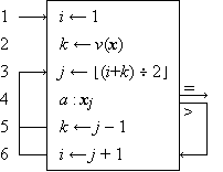Figure 1 Binary search

The entire process is described by the program appearing in Figure 1. The indices i and k are first set by steps 1 and 2 to include the entire list x. At each repetition of the loop beginning at step 3, the midpoint j is determined as the floor of the average of i and k. The three-way branch at step 4 terminates the process if x_j = a, and respecifies either the upper limit k or the lower limit i by branching to step 5 or to step 6 as appropriate. The convenience of the notation for the dimension of a vector in setting or testing indices is apparent from step 2.

Operations on Arrays

The convenience of extending the addition operator to vectors in a component-by-component fashion is well known. Formally,

is defined (for all numerical vectors x and y having a common dimension) by the relation z_i = x_i + y_i, for i = 1, 2, …, ν(x). In programming it is convenient to extend all of the basic operations on two variables in precisely the same way. For example, if x = (6, 3, 1, 4) and y = (1, 3, 5, 4),  then x + y = (7, 6, 6, 8),  x × y = (6, 9, 5, 16),  (x⌉y) = (6, 3, 5, 4),  (x > y) = (1, 0, 0, 0),  and (x > y)∨(x < y) = (1, 0, 0, 0)∨(0, 0, 1, 0) = (1, 0, 1, 0) = (x ≠ y).

Each of the basic operations are similarly extended element-by-element to matrices (e.g., X + Y,  X × Y,  (X ≠ Y), to yield a matrix result.

The summation of all components of a vector x is frequently used and is commonly denoted by ∑ x_i. In order to extend this type of process (called reduction) to all binary operations it is necessary to employ a symbolism which incorporates the basic operator symbol (in this case +), thus: +/x. For example, if x = (6, 3, 1, 4), and y = (1, 3, 5, 4), then +/x = 14, ×/x = 72, ⌉/x = 6 = –(⌋/(–x)), ∨/(x≠y) = 1, ∧/(x≠y) = 0, and +/(x≠y) = 2.

Reduction by a relation R is defined similarly:

For example, if x = (1, 0, 1, 1), then ≠/x denotes the application of the exclusive-or operation to x, and

The fact that an even-parity check (odd-parity codes are illegitimate) is equivalent to the exclusive-or may now be expressed (using the definition of residue from Table 1) as

≠/x = 2 | +/x.

Reduction of a vector by any operator is extended to a matrix M in two ways: to each of the rows (denoted by /M and called row reduction) or to each of the columns (denoted by //M and called column reduction). Each yields a vector result.

For example, if

	M =		0, 1, 1, 0		,  and N =		1, 0, 1, 1		,
			1, 1, 1, 0				1, 1, 1, 0
			0, 0, 1, 1				1, 0, 0, 1

then +//M = (1, 2, 3, l),  +/M = (2, 3, 2),  ≠/M = (0, 1, 0),  and ∧/(M=N) = (0, 1, 0).  Moreover, an even-parity check on all rows of M would be denoted by ∨/≠/M, and in this example a check failure would be noted, i.e., ∨/≠/M = ∨/(0, 1, 0) = 1.

Selection from Arrays

Although all elements of an array may normally receive the same treatment, it is frequently necessary to select subarrays for special treatment. The selection of a single element can be indicated by a subscript (e.g., x_i), but for the selection of groups of elements it is convenient to introduce the compression operation u/x. This is defined for an arbitrary vector x and a logical vector u of the same dimension:

y ← u/x

denotes that y is obtained from x by suppressing each component x_i for which u_i = 0. For example, if x_i = (d, e, s, i, g, n), and u_i = (1, 0, 0, 1, 1, 0), then u_i/x_i = (d, i, g). Moreover, (z ≠ y)/z denotes the selection from z of those components which differ from the corresponding components of y, and +/(z ≠ y)/z denotes the sum of such components. Operations are performed in order from right to left unless parentheses indicate otherwise.

Selection operations are extended to arrays in the same manner as reduction operations. Thus, if u = (1, 0, 1, 0), u = (1, 0, 1), and M and N are the matrices just employed in the examples of reduction, then

u/M = 0, 1 , 1, 1 0, 1

v//M = 0, 1, 1, 0 , 0, 0, 1, 1

N3/M = 0, 0 . 1, 1 0, 1

For example, if I is a 3 × 15 logical matrix representing the 3 index registers in a computer (e.g., the IBMB 7090), and if t is the 3-bit tag vector which selects the rows of I to be ored together to produce the vector z finally used in indexing, then

Certain essential operations converse to compression (mesh, mask, and expansion) are easily defined in terms of the compression operator itself and are extended to matrices in the established manner (Reference 1, p. 19).

To specify fixed formats it is convenient to adopt notation for several special logical vectors, each of a specifiable dimension n. Thus ⍺ ^j(n) denotes a prefix vector of j leading 1’s, ⍵ ^j(n) a suffix vector of j trailing 1’s, ∊ ^j(n) a unit vector with a 1 in position j , and ∊(n) a full vector of all 1’s. Hence, ⍺³(5) = (1, 1, 1, 0, 0), ⍵³(5) = (0, 0, 1, 1, 1), ∊²(4) = (0, 1, 0, 0), and (n) is a zero vector. If the dimension n is clear from compatibility requirements it may be elided. Thus, if c is the 36-bit command register of the IBM 7090 (which contains the next command to be executed), then ⍵¹⁵/c denotes the address portion.

Number Systems

The successive digits in the decimal representation of a number number such as 1776 may be treated as the components of a systems vector q = (1, 7, 7, 6) and the number they represent is then the base ten value of the vector q. More generally, a vector t may be evaluated in a mixed base system with radices specified by a radix vector r. This operation will be called the base r value of t and will be denoted by r ⊥ t. To define it by example, consider the system of temporal units up to the day, for which r = (24, 60, 60). Then if t = (2, 3, 4) is the elapsed time in hours, minutes and seconds, t = r ⊥ t = (2 × 60 × 60 + 3 × 60 + 4) = 7384 is the elapsed time in seconds.

In a fixed base b number system, r = b∊. Hence (10∊) ⊥ x is the base 10 value of x and (2∊) ⊥ y is the base 2 value of y. In the important case of base 2, elision of the radix vector 2∊ is permitted. Hence if the 2¹⁵ × 36 logical matrix M is the memory of the IBM 7090 and c is the command register, then

s ← M⊥⍵15/c.

describes the transfer of the operand to the storage register s.

If y is any number (not necessarily integral), then (y∊) ⊥ a obviously denotes the polynomial in y with coefficients a.

Permutation

A reordering of the components of a vector x is called permutation. Any permutation can be specified by a permutation vector whose components take on the value of its indices in some order. Thus, q = (3, 1, 4, 2) and r = (1, 4, 5, 2, 3) are permutation vectors. Permutation of x by a permutation vector p is denoted by x_p and defined as follows. If

y ← xp

then y_i = x_pi. For example, x_q = (x₃, x₁, x₄, x₂). It is clear from the definition that permutation is conveniently executed by indirect addressing.

Rotation is a particularly important case of permutation which warrants special notation. Thus k ↑ x denotes cyclic left shift by k places and k ↓ x denotes cyclic right shift. For example, 2 ↑ (t, e, a) = (a, t, e). Rotation of prefix and suffix vectors can be used to define infix vectors; e.g., 2 ↓ ⍺³(6) = (0, 0, 1, 1, 1, 0), and t = (18 ↓ ⍺³)/c denotes the index tag portion of the command c in the IBM 7090.

Permutation is extended to matrices by rows (X ^p) and by columns (X_p) in the established manner, as is rotation (k ↑ X and h X) .

Generalized Matrix Product

The ordinary matrix product, usually denoted by A B, can be defined conveniently using the reduction operation:

(A B)ji = +/(Ai × Bj).

To make explicit the role of the elementary operators + and ×, this product will be written as A B, and the definition will be extended more generally to A B,, where ₁ and ₂ are any pair of binary operators.

Applications of the generalized matrix product abound: if U is a square logical matrix representing the direct connections in a network (node i is connected to node j if U_jⁱ = 1), then M = U U is the matrix of connections via paths of length two; if D is a distance matrix (D_jⁱ is the direct distance from city i to city j), then T = D D is the matrix of distances for the shortest trip of exactly two legs. The well-known identities of matrix algebra can be easily and usefully extended to operators other than ().
 

Conclusion

In comparing this programming language with others, it is necessary to consider not only its use in description and analysis (which has been emphasized here), but also its use in the execution of algorithms, i.e., its use as a source language to be translated into computer code for the purpose of automatic execution.

In description and analysis (and hence in exposition), the advantages over other formal languages such as FORTRAN and ALGOL reside mainly in the conciseness, formalism, variability of level, and capacity for systematic extension.

The conciseness and its utility in the comprehension and the debugging of programs are both fairly obvious. The advantage of formalism (i.e., of numerous formal identities) in a programming language is not so clearly recognized. Programme 2 of Reference 3 provides an example of the use of formal identities in establishing the behavior of an algorithm; a similar treatment could easily be provided for Program 2 (matrix inversion by Gauss-Jordan) of Reference 2. Indeed, any valid algorithm for a specified process is itself an outline of a formal constructive proof of its own validity, the details being provided by the formal identities of the language in which the algorithm is presented.

The ability to describe a process at various levels of detail is an important advantage of a language. Reference 2 illustrates this ability in the specification of a computer; Programs 6.32 and 6.33 of Reference 1 illustrate it at a quite different level, involving the description of the repeated-selection sort in terms of tree operations and in terms of a representation of the tree suitable for execution on a computer.

The capacity for systematic extension is extremely important because of the impossibility of producing a workable language which incorporates directly all operations required in all areas of application; the best that can be hoped for is a common core of operations which can be extended in a systematic manner consistent with the core. As a simple example, consider the introduction of exponentiation. Since this is a binary operation, an operator symbol, say , is adopted and is used between the operands; thus yx denotes x raised to the power y. Then yx, YX, /x, etc., are automatically defined. As a further example, consider the adoption (in the treatment of number theory) of operators for greatest common divisor (xy) and for least common multiple (xy). Then /x is the g.c.d. of the numbers x₁, x₂, … x_ν. Moreover, if p is the vector of the first ν(p) primes (e.g., p = (2, 3, 5, 7, 11)), and f is the vector of exponents in the prime factorization of a number n, then n = fp. Similarly, if F ⁱ is the factorization of n_i, then n = Fp, and clearly, /n = (⌋//F)p, and /n = (⌉//F)p.

Compared to ordinary English, this notation shares with other formal languages the important advantage of being explicit. Moreover, it is rich enough to provide a description which is as straightforward as, and easily related to, the looser expression in English. For example, indirect addressing (via a table of addresses p) is denoted by x_pi.

In the matter of execution, the advantages of this notation in analysis and exposition are, in some areas at least, sufficient to justify its use even at the cost of a subsequent translation (to another source language for which a compiler exists) performed by a programmer. However, for direct use as a source language, two distinct problems arise: transliteration of a program in characters available on keyboards and printers, and compilation.

Because operator symbols were chosen for their mnemonic value rather than for availability, most of them require transliteration. However, because the symbols are used economically (e.g., the solidus “/” denotes compression as well as reduction, the symbol-doubling convention eliminates the need for special symbols for column operations, and the relational statement obviates special operators for exclusive-or, implication, etc.) the total number of symbols is small. (Note that the set of basic symbols employed in a language such as ALGOL includes each of the specially defined words such as IF, THEN, etc.)

Operator   Symbol (   ( )   ) ←   $ ∨   + ∧   *   –X +   @+ ×   @* –   @– ÷   D

Operator   Symbol ⌈X⌉   C X ⌊X⌋   F X |   R M =   = ≠   @= >   G <   @G /   / \   @/   ,

Operator   Symbol ⊥   B ↑   L ↓   R ⍺ j   A J ⍵ j   W J ε   E ⍳j   I J μ   M ν   N

Reference 4 outlines one of many possible simple transliteration schemes. The mnemonic value of the original symbols must be sacrificed to some extent in transliteration, but the transliteration need not impair the structure of the language—a matter of much greater moment.

The complexity of the compilation of a source language is obviously increased as the language becomes richer in basic operations, but is decreased by the adoption of a systematic structure. The generalized matrix product XY, for example, greatly increases the power of the source language, but the compiler need produce only the same skeleton program required for the ordinary matrix product, permitting the specification of ₁ and ₂ as any of the basic operations in its repertoire. Moreover, the direct provision of array operations frequently simplifies rather than complicates the task of the compiler. For example, the operation XY could be compiled so as to execute the basic arithmetic operations in any one of several orders and could therefore choose one best suited to the indexing and other facilities available. On the contrary, the use of DO statements as in FORTRAN or ALGOL, although it requires the programmer to specify more detail (i.e., the indexing), makes it difficult or impossible for the compiler to determine whether the particular order of execution specified by the indexing of the loops is essential, and hence inviolable.

In this brief exposition it has been impossible to explore many extensions of the notation such as set operations, files, general index-origins, and directed graphs and trees. Likewise, it has been impossible to include extended examples. However, a mastery of the simple operations introduced here should permit the interested designer to try the notation in his own work, referring to the papers indicated in the bibliography for extensions of the notation and for guidance from its previous use in applications similar to his own. The portion of the notation essential to microprogramming is summarized in Table 1.
 

Acknowledgment

I am indebted to Mr. A.D. Falkoff, Mr. A.L. Leiner, Professor A.G. Oettinger, and the Journal referees for helpful comments arising from their reading of the manuscript.
 

Cited References

Bibliography