Recreational APL
Eugene McDonnell
December 1977
The Story of ○
| The circle is a perfect thing. | |
| — Aristotle De Caelo,I,2 | |
| “...many different notations for the circular and hyperbolic functions were entertained over a period of more than a year before the present scheme was proposed, whereupon it was quickly adopted.” | |
| — Falkoff and Iverson [2] |
To facilitate working with complex numbers,
proposals were made at the APL Minnowbrook Workshop
last September to augment the number
of left arguments to the dyadic circle function.
My principal purpose in this article is
to describe several of those proposals.
Before doing that, however,
I’ll give you the history of the circle notation in APL.
History
After the initial implementation of APL\360 in November 1966, the lack of a suitable notation for the trigonometric functions and their inverses was felt very strongly. There was no difficulty in obtaining accurate and efficient algorithms, since the excellent subroutines developed by the late Hirondo Kuki of the University of Chicago were available.
In Iverson’s 1962 book [3], there are two fleeting uses of the trigonometric functions. In both places they relate not to functions on real numbers, but rather to dyadic functions between vector arguments. In the first instance [3, p.40], the notation “Cos(x,y)” is used as the name of a subroutine that determines z as the cosine of the angle between the vectors x and y . In the second instance [3, p. 70], the notations xγy and xσy are used to describe dyadic functions that give the cosine and the sine, respectively, of the angle between the vector arguments x and y .
In Iverson’s 1966 book [4], there is a development from the exponential function *x to a function Ax that is the average of *x and *-x , and then to a function Bx that is half the difference of *x and *-x , and finally to two functions that can be obtained by reversing the signs of alternate nonzero terms of the series expressions for Ax and Bx . The first of these is denoted Cx , while the second (are you following?) is denoted Sx .
Of course, it develops that the functions Cx and Sx are the cosine and sine functions. Ax and Bx are shown to be the hyperbolic cosine and hyperbolic sine functions, and two other notations, Tx and Ux , are employed for the tangent and hyperbolic tangent functions.
In this book
[4],
the notation for an inverse function was obtained
by adding a prime sign to the notation for the function.
Thus, the logarithm function was denoted by *'
and the arctangent function by T' .
Also, the reciprocal of a function was denoted by an overbar.
The secant function was denoted
by  ,
and the cotangent
by
,
and the cotangent
by  .
.
APL\360 followed shortly after the appearance of this book. By the time it appeared, the typography of APL had taken on some definite characteristics. In particular, each primitive function was denoted by a nonalphabetic symbol. It was strongly felt by the language designers that alphabetic notations, such as sin , cos , S , or C , should not be used for primitive functions. Furthermore, inverse functions were acquiring their own symbols, for example, the logarithm function being denoted by ⍟ rather than *' . (By the way, there is a visual pun here — this symbol looks like the cross-section of a felled tree, that is, a log.)
This meant that the three trigonometric functions, their inverses, their reciprocals, and the inverses of the reciprocals, and then the same panoply for the hyperbolic functions, all were lacking notations — 24 functions in all. In the meantime, the complaints from users who were having to define functions or copy defined functions from a workspace when they needed a trigonometric function were pouring in. I still have copies of some of these defined functions, found in early public libraries. These were generally not particularly efficient nor were they very accurate.
There was thus a good deal of dissatisfaction with the situation. The proposal being considered in early Spring 1968 was to use the monadic forms of the six relational functions (< ≤ = ≥ > ≠) for the sine, cosine, tangent, and their inverses, and the same symbols, overstruck with the dieresis, for the hyperbolic functions and their inverses. No one was particularly happy with this design.
It was at this point that I put three thoughts together, and invented what Paul Penfield has so aptly called “this arbitrary and slightly distasteful” notation [5]. The first thought was a principle enunciated by Iverson in his first book [3, p. 8]:
| A concise programming language must incorporate families of operations whose members are related in a systematic manner. Each family will be denoted by a specific operation symbol, and the particular member of the family will be designated by an associated controlling parameter ... which immediately precedes the main operation symbol. The operand is placed after the main operation symbol. |
This gave the method of unifying the members of a family of functions, but it lacked two things: the values of the controlling parameters and the operation symbol.
The second thought determined the values of the controlling parameters, by recalling that the sine and the tangent functions were odd functions, as were the hyperbolic sine and hyperbolic tangent. This suggested that odd numbers be used to designate them. The values 1 , 3 , 5 , and 7 seemed appropriate. (An odd function is one for which F-x is equal to -Fx . Signum is an odd function, for example; ×-5 is equal to -×5.)
Actually, 1 and 3 were chosen first, more or less by accident, for the sine and tangent, along with 2 for the cosine function, by listing the functions in the order in which they were taught me in high school, and then the observation was made about sine and tangent being odd functions. The hyperbolic functions simply fell into place afterwards.
Also, cosine is an even function. (An even function is one for which F-x is equal to Fx . The magnitude function is even; |-5 is equal to |5 .) Thus the 2 , which had been associated with the cosine, turned out to have some mnemonic value. This burgeoning correspondence between control parameter value and odd and even functions led to the assignment of control parameter value 6 to the hyperbolic cosine function, also an even function.
The availability of the negative integers made the determination of control parameter values for the inverse functions (arcsine and so on) simple. This left three gaps in the numbering scheme — at ¯4 , 0 , and 4.
The third thought had to do with the function symbol. In the layout of the APL printing element, several symbols had been put on it in order to be used with other symbols: the dieresis, overbar, underbar, quad, and circle. Nevertheless, when a symbol for the circular function notation was needed, what better symbol than the circle by itself? This was proposed and ultimately accepted. There were some feelings that it would not make a very good symbol for hand exposition (say, at a blackboard), but there was such a right feeling about it that this objection was overcome.
The monadic use of the circle notation was part of the initial proposal. There was already a way to obtain the useful constant e , namely *1 , but no way to obtain that equally useful constant pi. So the monadic use of the circle was used to denote multiplication by pi. Iverson toyed briefly with the notion of having this monadic use mean division by pi, but eventually decided that multiplication by pi had just as strong a claim, if not a greater one, to be the monadic significance.
The original proposal for the gaps at ¯4 , 0 , and 4 was to assign to them (redundantly) the meanings logarithm, pi times, and exponential. Logarithm and exponential are neither odd nor even, and pi times is odd, whereas 0 is even, but these functions occur so frequently in combination with the others that it was thought they would have some marginal use.
On the day after the meeting at which this proposal was laid before Ken Iverson, Adin Falkoff, and Larry Breed, Breed called an emendation meeting. He suggested that we discard the assignments proposed for ¯4 , 0 , and 4 . In their place, he suggested that we retain the parity scheme for the functions to be associated with these control parameter values, that the functions assigned to ¯4 and 4 be inverses, and that the function assigned to 0 be self-inverse. Furthermore, these functions should be allied with the circular and hyperbolic functions. In fact, he proposed the functions that are now associated with these numbers.
At that point the suggestion was made that we needn’t stop there: that functions could be associated with parameter values 8 and up. In fact, the functions (x-1)÷x+1 and (1+x)÷1-x were inverses, and could be associated with 8 and ¯8 . It was at this point that Iverson and Falkoff decided to be quite cautious about enlarging the left domain of this function. To quote from [2]:
| The notational scheme employed for the circular functions must clearly be used with discretion; it could be used to replace all monadic functions by a single dyadic function with an integer left argument to encode each monadic function. |
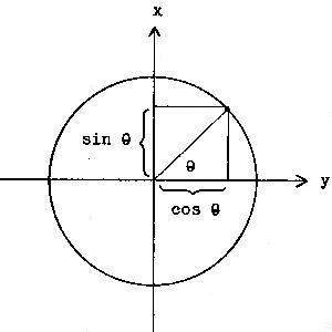
I do not know whether anyone who participated in this design session was aware that the digit 1 is vertical, whereas the digit 2 has a strong horizontal base, and that the sine function relative to the unit circle in the Cartesian plane is depicted vertically, and the cosine function is shown horizontally. But remember that.
The news of this notation was communicated to a group at Science Research Associates in Chicago which was working on an implementation of APL for the IBM 1500 computer. In a few days they had implemented all of the functions. This group included Harold Driscoll, Scott Kreuger, and Tom McMurchie. To them goes the distinction of having provided the first implementation of APL’s circular functions. Not far behind, the group at Watson Research in Yorktown Heights, New York, had them implemented a week later. We had to wait for K. M. Brown, then of Cornell University, to design algorithms for some of the hyperbolic functions.
The ¯4 , 0 , and 4 circle functions went nameless for years. Not until APL Language (IBM publication GC26-3847) was being prepared in early 1975, did it occur to me that since these were intimately related to the theorem of Pythagoras and in fact dealt with the catheti and hypotenuse of right-angled triangles having one unit-length leg, it was possible to call them the Pythagorean functions. This was proposed to Iverson, with the consequence that this IBM manual has a section in it with the resounding title, “The Circular, Hyperbolic, and Pythagorean Functions”.
I wish I could tell you how endlessly useful these functions have been to users of APL. Instead I have to confess that, though most of these are essential functions for any general purpose programming language, in the general run of applications they are not used very much at all. In Bingham’s static analysis of APL programs [1], the dyadic circular functions are lumped together with general logarithm, binomial, nand, and nor as “other”, and this entire group represents only 1.2% of all dyadic scalar functions and 0.1% of all tokens. Similar statistics have been obtained for the monadic circle function.
Another incident indicates the frequency
of use of some of the circular functions.
Someone called me in Palo Alto from the IBM plant in Endicott, New York,
one day to say that the inverse hyperbolic tangent function
did not appear to be giving proper results for nonscalar arguments.
I verified that the report was true,
and found that, sure enough,
a register that should have been preserved
by this function was destroyed,
not by the function itself but
by the square root subroutine it called.
The requirement for preserving the register had arisen
when Jim Brown’s scalar function compiler had appeared,
in release 3 of APLSV.
Earlier versions of APLSV had not had this compiler facility.
Now, release 3 of APLSV had been in daily use by tens of thousands
of users at many, many locations,
inside IBM and at customer sites,
for over six months before this bug was found.
No customer ever experienced it, to my knowledge.
So much for the utility
of the inverse hyperbolic tangent function.
Some Problems
| 1. |
The formula for the area of a circle or for the volume
of a sphere can be generalized to give the hypervolume
of a hypersphere in n-space for any positive n .
For a unit radius hypersphere,
the hypervolume for dimension ⍵ is given by
nvol:(2÷⍵)×((○1)*.5×⍵))÷!¯1+.5×⍵ What dimension of space gives the maximum hypervolume
to the unit radius hypersphere? | |
| 2. | Since 2○0 is 1 and 2○○÷2 is 0 , there must be a value of the argument to cosine that is equal to its own cosine. What is a simple way to compute this value? |
The New Proposals
Penfield’s paper [5] appeared in the September 1977 issue of Quote Quad and also was distributed to those attending the Minnowbrook APL Workshop. Since no session was scheduled to discuss his paper, he and I organized a special session during free time one afternoon. This special session had to compete not only with people’s desire to relax, but with the only sunshine of the three days and a floatplane taking passengers for tours at the dock near the classroom (and visible from the classroom windows). It is some indication of the interest in this topic that about half of the attendees gave up those other attractions to listen to the talk Penfield gave on his paper.
He reports elsewhere in this issue on the overall subject of complex numbers in APL (see “Extension of APL Primitive Functions to the Complex Domain”). Here I shall report only on some recommendations that came from this meeting concerning notation for functions to provide the real and imaginary parts and the magnitude and arc of a complex number.
On all of the schemes proposed in Penfield’s paper, a consensus was quickly reached that the fifth showed the greatest promise. This proposal provided the additional left arguments for the dyadic circle function of 8 , 9 , 10 , and 11 , in order to signify the real part, imaginary part, magnitude, and arc, respectively. Suitable inverses were proposed for the negatives of these values. There was, however, the feeling that these assignments appeared to be quite arbitrary, and lacked any mnemonic significance.
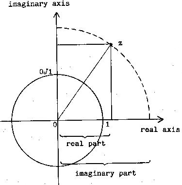
Glen Seeds of MCM, Ltd., made an interesting observation and a suggestion. He pointed out that we could exploit the fundamental similarity of the Cartesian plane and the complex plane. Just as in the Cartesian plane, the sine is related to the vertical displacement of a point on the unit circle, and the cosine to the horizontal displacement, so in the complex plane, the imaginary part is related to the vertical displacement of a point with respect to the real axis, and the real part is related to the horizontal displacement of a point with respect to the imaginary axis.
Seeds suggested that we exploit the similarity between the planes in providing new left arguments for the dyadic circle function. In particular, he suggested we correlate the imaginary part function with the sine function by assigning 11 as the left argument that denotes the imaginary part function — 11 being 10 more than the argument that denotes the sine function; he also suggested we denote the real part function by left argument 12 , that is, 10 more than the argument that denotes the cosine function.
This scheme continues, Seeds noted, as we seek appropriate left arguments to denote the arc function and its companion, the magnitude function. The arc function (which Penfield calls the phase function) is computed, for nonzero arguments, as the arctangent of the ratio of the imaginary part to the real part. We could denote this function with left argument 13 , that is, 10 more than the argument that denotes the tangent function. Finally, the magnitude function is defined as the positive square root of the sum of the squares of the real and imaginary parts. We could normalize this by factoring out, say, the real part, as the product of the real part and the 4 circle function of the ratio of the imaginary and real parts. Thus we have some justification, and a mnemonic device, for associating the left argument 14 with the magnitude function. The inverses for these functions would be essentially as given by Penfield’s fifth proposal.
To summarize Glen Seed’s memorable suggestion, the chart for the circle functions under this scheme would be augmented with four more rows:
| (-a)○b | a | a○b | |||
| ------ | - | --- | |||
| 0j1×b | 11 | Imag b | |||
| +b | 12 | Real b | |||
| *0j1×b | 13 | Arc b | |||
| b | 14 | Magnitude b |
These proposals brought the unplanned meeting to a close. However, it wasn’t very long before the gap in the series, between 7 and 11 , was noticed. What should we do with 8 , 9 , and 10 ? We couldn’t just leave them unassigned, could we?
The next suggestion rather startled me, since I had proposed it nine years earlier as the meanings to be assigned to 4○b and ¯4○b : and that was to use one of the unassigned numbers to signify the exponential of the right argument, and the negative of that number to signify the natural logarithm of the right argument. Another number could be used to signify the reciprocal of the right argument. Since reciprocal is self-inverse, the negative would have the same meaning. These proposals were both made, I believe, by Ken Iverson. He said their utility would be found in producing expressions involving multiple uses of the dyadic circle function, since so often reciprocals, exponentials, and logarithms appear in conjunction with the existing circular functions.
Seeing the resurrection of these old nominations, I ventured to suggest the functions (b-1)÷b+1 and (1+b)÷1-b as another candidate pair. Imagine my surprise when Penfield, first of all, recognized these immediately as a bilinear transformation and its inverse (I didn’t know their names), and, secondly, thought that they would be of utility in the complex domain. The circumstance seems to be that this bilinear transformation is one of the common transformations of the complex plane, mapping the right half-plane into the interior of the unit circle, and the interior of the unit circle into the left half-plane.
All of this took place within a few hours of the breaking-up of the unscheduled session. The following new assignments were proposed:
| (-a)○b | a | a○b | |||
| ------ | - | --- | |||
| (1+b)÷1-b | 8 | (b-1)÷b+1 | |||
| ⍟b | 9 | *b | |||
| ÷b | 10 | ÷b |
These three assignments were made with
less certainty than the earlier four had been.
And Now for the Fun
That night, after dinner and the evening session (which broke up at 9:30), several people sat in the back of the pleasant lounge area, as the fireplace crackled and the musicians and singers began assembling. One person mentioned that during the afternoon meeting it had been seriously proposed that a variation of the arc function be provided which gave a result in degrees rather than radians. This was really not such a bad proposal, but it led to many bad ones. For example, how about 16○b to convert from radians to degrees, and ¯16 from degrees to radians? And then, what about 17○b which converted b from degrees Celsius to degrees Fahrenheit?
I suggested, not completely in jest, that 19○b convert its argument from Julian day number to Gregorian date, a three-element vector. The inverse ¯19○b would require a three-element vector argument and would produce the corresponding Julian day number.
This led to 20○b , which converts b from a Gregorian date to a day of the week, expressed as a value in the range ⍳7 (origin-dependent). A new system variable ⎕rp (religious preference) would allow the user to specify whether the week begins on Saturday or Sunday (or any other day). The inverse function ¯20○b is not unique, and a principal value would have to be determined in order to give a unique result. We would need a canonical Monday, Tuesday, and so on.
This could easily be run into the ground, so I will spare you most of the rest of the night’s ingenuity. What about 18 , did you ask? Oh yes! 18○b would convert b from an Arabic number to a Roman number. Then the inverse function, to convert from a Roman number to an Arabic number, would of course be given by ¯xviii○b .
Thus the night ended, and we went off to sleep telling each other that the cold light of dawn would help us determine whether the day’s work had been all nonsense or just the late night part.
The morning came, and much to everyone’s surprise, the serious discussions of the previous day held up quite well. There was, unfortunately, one further addition to the nonsense of the night before that I cannot forbear inflicting on you. Fortunately you have to be up on the recondite conflicts in array theory for the thing to have any point, so most of you will be spared it. I shall conceal the identity of the perpetrator.
The function 108○b takes an integer right argument from the set of elements 0, 1, and 2, and gives as result a character vector which is a description of array theory according to axiom system 0, 1, or 2. The inverse function ¯108○b takes a character string right argument, purporting to represent a description of array theory, and the result is 0, 1, or 2, according to which axiom system the description corresponded.
As we broke up the meeting, Louis Robichaud was assuring people
that he would have circular
functions 8 through 14 implemented
by the following Monday back at Laval University.
No one dared to doubt him.
References
| 1. | Bingham, H.W. Content analysis of APL defined functions. APL 75 Congress Proc. (Pisa), ACM, New York, 1975, pp. 60-66. | |
| 2. | Falkoff, A.D., and Iverson, K.E. The Design of APL. IBM Journal of Research and Development 17 (1973). | |
| 3. | Iverson, K.E. A Programming Language. Wiley, New York, 1962. | |
| 4. | Iverson, K.E. Elementary Functions. Science Research Associates, Chicago, 1966. | |
| 5. | Penfield, P., Jr. Notation for complex “part” functions. APL Quote Quad 8, 1, (Sept. 1977), 11-13. |
Puzzle of the Year, 1978
An anonymous contributor sent in the following challenging problem:
The start of the new year is a good time for a series of one hundred puzzles using the digits 1 , 9 , 7 , and 8 . For each number n from 1 through 100 , write an APL expression, as short as possible, using no letters and no digits except those four, which must appear in the same order (1 , 9 , 7 , 8) with other APL characters interspersed. The result must be a scalar.
For example, consider n=1 . The expression 1 97[×8] works, but requires eight characters. Surely we can do better. The expression ⍴,1978 is disqualified because it is a vector, not a scalar. The expressions ⌈19÷78 and ~197!8 and ⌊1.978 have length six. Solutions of length five include 19≠78 and ×l978 and 197≥8 and 1⌊978 .
The lengths of the shortest expressions known so far are listed below. Only six of these are of the minimum length, five; all others represent opportunities for improvements from readers. See how many of these lengths you can achieve, and send in your solutions if they are of shorter length.
      10 10⍴lengths
 5  5  7 7 7 6 6 5 6  6
 6  9  8 8 6 7 7 6 5  6
 7  8  7 6 6 6 6 8 8  8
 8  8  8 6 8 8 7 8 8  8
 8  7  7 8 8 9 8 8 9  9
 8  8  8 9 9 6 7 9 6  7
 8  7  7 7 9 8 8 7 7  6
 8  7  7 8 6 8 7 5 6  8
 8  7  7 8 8 7 6 6 6  6
10 10 10 7 7 7 5 6 7 10
First appeared in
APL Quote-Quad, Volume 8, Number 2, 1977-12.
The text requires the APL385 Unicode font, which can be
downloaded from
http://www.vector.org.uk/resource/apl385.ttf .
To resolve (or at least explain) problems with displaying
APL characters see
http://www.vector.org.uk/archive/display.htm .
last updated: 2009-11-23 18:55